Group Convolution Neural Networks

TL;DR: This blog introduces group convolutional neural networks (Group CNNs) [1,2], which guarantee symmetries in neural networks; for example, a rotated cat is guaranteed to be classified as a cat under Group CNNs, i.e., symmetries over the rotation group. It aims to simplify abstract concepts for newcomers. Coding examples are provided to illustrate these concepts. The code is much simpler compared to complex libraries, but it includes the essential functionalities needed to grasp the underlying concepts.

• The toy implementation along with some slides can be found here.

1. Introduction

1.1. Why Symmetries

Group equivariance in ML models is about enforcing symmetries in the architectures.

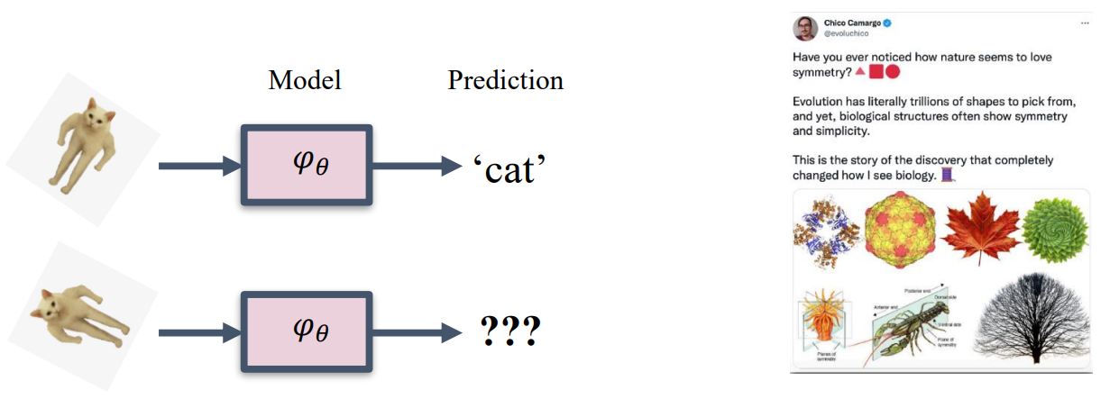
• Many learning tasks, oftentimes, have symmetries under some set of transformations acting on the data.
  • For example, in image classification, rotating or flipping an image of a cat should not change its classification as a “cat.”
• More importantly, nature itself is about symmetries.
  • Similar symmetries appear in physical systems, molecular structures, and many other scientific data.

FYI: Dr. Chen Ning Yang from Stony Brook received the Nobel Prize in physics (1957) for discoveries about symmetries, and his B.S. thesis is “Group Theory and Molecular Spectra”.

1.2. Learning Symmetries

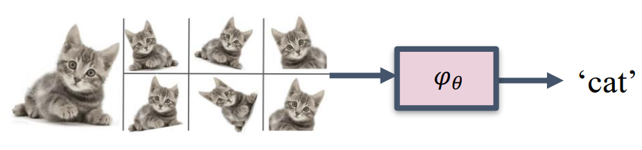
To learn symmetries, a common approach is to use data augmentation: feed augmented data and hope the model “learns” the symmetry.

Issues:

• No guarantee of having symmetries in the model
• Wasting valuable net capacity on learning symmetries from data
• Redundancy in learned feature representation

Solution:

• Building symmetries into the model by design!

2. Mathematical Preliminary

2.1. Definition: Group

A group $(G, \cdot)$ is a set of elements $G$ equipped with a group product $\cdot$, a binary operator, that satisfies the following four axioms:

• Closure: Given two elements $g$ and $h$ of $G$, the product $g \cdot h$ is also in $G$.
• Associativity: For $g, h, i \in G$ the product $\cdot$ is associative, i.e., $g \cdot(h \cdot i)=(g \cdot h) \cdot i$.
• Identity element: There exists an identity element $e \in G$ such that $e \cdot g=g \cdot e=g$ for any $g \in G$.
• Inverse element: For each $g \in G$ there exists an inverse element $g^{-1} \in G$ s.t. $g^{-1} \cdot g=g \cdot g^{-1}=e$. Example:

The translation group consists of all possible translations in $\mathbb{R}^2$ and is equipped with the group product and group inverse:

with $g=(t), g^{\prime}=\left(t^{\prime}\right)$, and $e=(0,0)$.

2.2. Definition: Representation and Left-regular Representation

A representation $\rho: G \rightarrow G L(V)$ is a group homomorphism from $\mathrm{G}$ to the general linear group $G L(V)$. That is, $\rho(g)$ is a linear transformation parameterized by group elements $g \in G$ that transforms some vector $\mathbf{v} \in V$ (e.g. an image or a tensor) such that

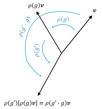
This essentially means that we can transfer group structure to other types of objects now, such as vectors or images.

Note:

• A homomorphism is a structure-preserving map between two algebraic structures of the same type (such as two groups, two rings, or two vector spaces).
• A general linear group is the group of all invertible $d_V \times d_V$ matrices.

A left-regular representation $\mathscr{L}_g$ is a representation that transforms functions $f$ by transforming their domains via the inverse group action

Example I:

• $f \in \mathbb{L}_2\left(\mathbb{R}\right)$: A function defined on a line.
• $G=\mathbb{R}$: The 1D translation group.
• $[\mathscr{L}_{g = t}f]~(x)=f\left(t^{-1}_θ \odot x\right) = f(x - t)$: A translation of the function.

Example II:

• $f \in \mathbb{L}_2\left(\mathbb{R}^2\right)$: A 2D image.
• $G=S E(2)$: The 2D roto-translation group.
• $[\mathscr{L}_{g = (t, \theta)}f]~(x)=f\left(\mathbb{R}^{-1}_θ (x-t)\right)$: A roto-translation of the image.

Remark: Now we have group stucture on different objects

1. Group Product (acting on $G$ it self): $g\cdot g’$
2. Left Regular Representation (acting on a vector spaces): $\mathscr{L}_gf$
3. Group Actions (acting on $\mathbb{R}^d$): $g \odot x$

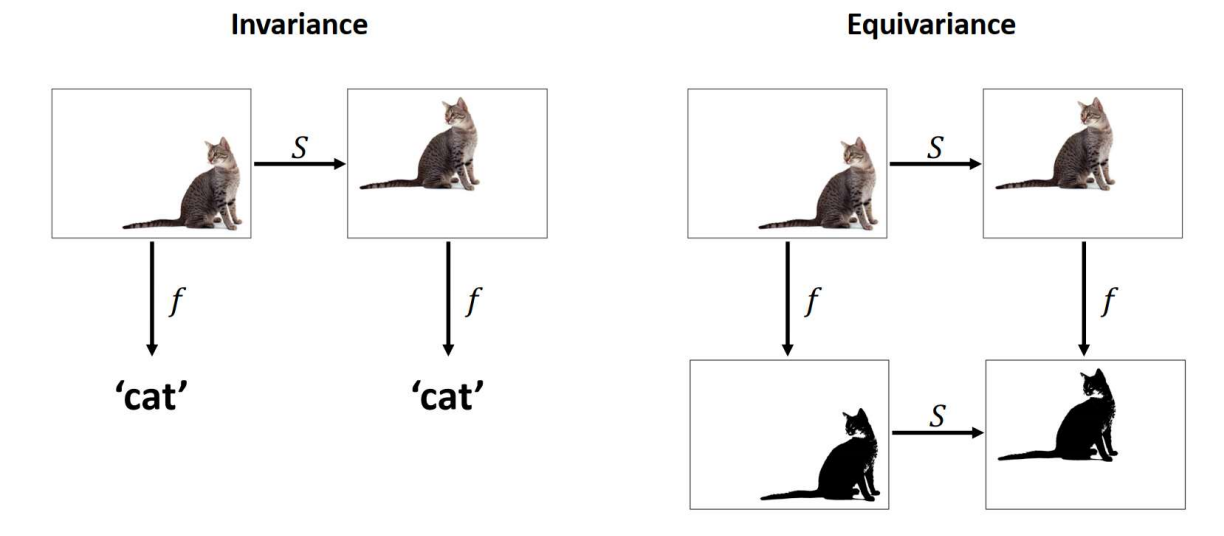
2.3. Definition: Equivariance and Invariance

Equivariance is a property of an operator $\Phi: X \rightarrow Y$ (such as a neural network layer) by which it commutes with the group action: \(\Phi \circ \rho^X(g)=\rho^Y(g) \circ \Phi,\)

Invariance is a property of an operator $\Phi: X \rightarrow Y$ (such as a neural network layer) by which it remains unchanged after the group action:

• $\rho^X(g)$: group representation action on $X$
• $\rho^Y(g)$: group representation action on $Y$
• Invariance is a special case of equivariance when $\rho^Y(g)$ is the identity.

3. CNNs and Translation Equivariance

3.1. Convolution and Cross-Correlation

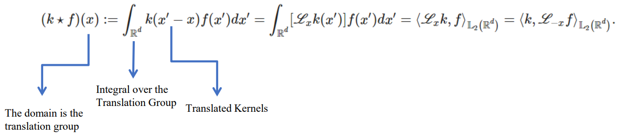
The convolution of $f$ and $g$ is written as $f * g$, denoting the operator with the symbol $*$. It is defined as the integral of the product of the two functions after one is reflected and shifted. As such, it is a particular kind of integral transform:

An equivalent definition is (commutativity):

The corss-correlation of $f$ and $g$ is written $f \star g$, denoting the operator with the symbol $\star$. It is defined as the integral of the product of the two functions after one is shifted. As such, it is a particular kind of integral transform:

An equivalent definition is (not commutativity in this case):

Note: Neural networks perform the same whether using convolution or correlation because the learned filters enable adaptability. The filters are learned, and if a CNN can learn a task using the convolution operation, it can also learn the same task using the correlation operation (it would learn the rotated version of each filter).

3.2. Translation Equivariance

Convolution and cross-correlation are translation equivariant, so are their discrete counterparts.

Proof:

1. Translate $f$ by $t$ first, then apply the convolution:

1. Apply convolution first, and then translate by $t$:

In the last equality, we just replace $x’$ by $x’ - t$. Note that this operation is valid because this substitution is a bijection $\mathbb{R}^d \rightarrow \mathbb{R}^d$, and we integrate over the entire $\mathbb{R}^d$.

By similar arguments, we can prove translation equivariance for convolution and its discrete versions.

3.3. Intuition on Translation Equivariance

Mathematically, it is easy to prove translation equivariance. However, let’s look at the definition of cross-correlation again to gain some intuition about how to achieve equivariance.

Cross-Correlation:

Replace $x’$ by $x’+x$:

Intuition:

• $f(x’ + x)$ represents a translated version of $f(x)$. We have created many translated versions of $f(x)$ while creating the feature map. If we need to compute the cross-correlation for a transformed $f$, we can just go and look up the relevant outputs because we have already computed them. Equivalently, $k(x’ - x)$ represents a translated version of $k(x)$.
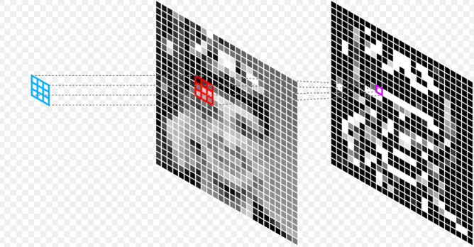
• In CNNs, we translate the kernel across the image to “scan” the image.

3.4. Generalization

Let’s look at the definition of cross-correlation:

Here, we explicitly think of the cross-correlation in terms of translations. To generalize, if we want to transform $f$ with other groups, the trick is to make the kernel $k$ be represented by a group. Group representations on $k$ are reflected on $f$ as well.

To generalize to other groups, we should consider the following:

• Make the function defined on the group of interest.
• Integrate over the group of interest.
• Make the kernel reflect the actions of the group of interest.

4. Regular Group CNN and $SE(2)$ Equivariance

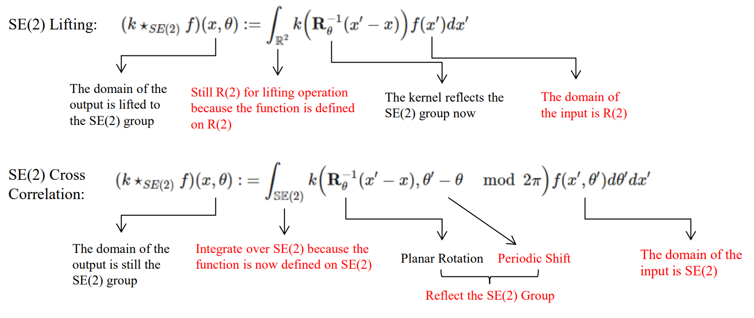
4.1. Definition: $SE(2)$ Lifting Correlation

To make the function defined on the group of interest, we define the lifting operation. The lifting correlation of $f$ and $g$ is written as $f \star_{SE(2)} g$, denoting the operator with the symbol $\star_{SE(2)}$. It is defined as the integral of the product of the two functions after one is shifted and rotated. As such, it is a particular kind of integral transform:

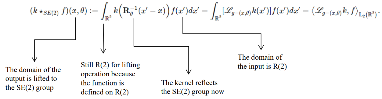
Lifting correlation raises the feature map to a higher dimension that represents rotation. Now, planar rotation becomes a planar rotation in the $xy$-axes and a periodic shift (translation) in the $\theta$-axis.

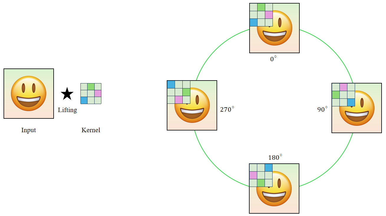
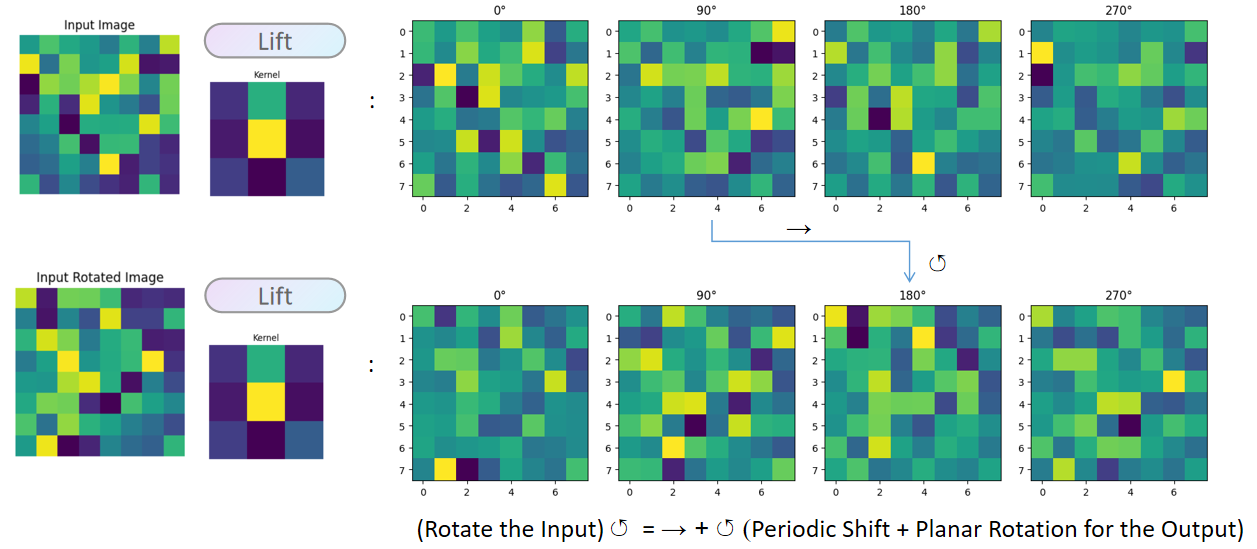
4.2. Demonstration: Lifting Correlation with the $p_4$ Rotation Group

The $p_4$ group can be described as a semi-direct product:

where:

• $C_4$ : The cyclic group of order 4 representing the rotational symmetries.
• $\mathbb{Z}^2$ : The group of translations in the plane (not $\mathbb{R}^2$ because images are discrete).

The lifting operation will simply convolve the input with the kernels rotated by $0^\circ$, $90^\circ$, $180^\circ$, and $270^\circ$, respectively. The result contains $4$ feature maps that correspond to these angles.

def lift_correlation(image, kernel):
    """
    Apply lifting correlation/convolution on an image.

    Parameters:
    - image (numpy.ndarray): The input image as a 2D array, size (s,s)
    - conv_kernel (numpy.ndarray): The convolution kernel as a 2D array.

    Returns:
    - numpy.ndarray: Resulting feature maps after lifting correlation, size (|G|,s,s)
    """
    results = []
    for i in range(4):  # apply rotations to the kernel and convolve with the input
        rotated_kernel = np.rot90(conv_kernel, i)
        result = convolve2d(image, rotated_kernel, mode='same', boundary='symm')
        results.append(result)
    return np.array(results)

The resulting feature maps in the group space are equivariant (rotation in the input $\mapsto$ planar rotation + periodic shift in the output features).

4.3. Definition: $SE(2)$ Group Cross Correlations

Now, the function is already defined on the group of interest after lifting. We still need to convolve over the group of interest and make the kernel reflect the actions of the group of interest.

The group correlation of $f$ and $g$ is written as $f \star_{SE(2)} g$, denoting the operator with the symbol $\star_{SE(2)}$. It is defined as the integral of the product of the two functions after one is shifted and rotated:

Although the examples are given for the group $\mathrm{SE}(2)$, the idea can generalize to other affine groups (semi-direct product groups).

If we look carefully at how rotational equivariance is achieved, we find that it basically adds a rotation dimension represented by an axis $\theta$. Thus, the rotational equivariance problem now becomes a translation equivariance problem, which can be solved easily by convolution/cross-correlation.

Note: Translations and $H$-transformations form so-called affine groups: $\operatorname{Aff}(H) := \left(\mathbb{R}^d, +\right) \rtimes H.$

4.4. Demonstration: Cross Correlation with the $p_4$ Rotation Group

Now, we have to reflect the differences in formulation between the lifting correlation and cross-correlation in the code as well.

def p4_group_convolution(features, kernel):
    """
    Perform P4 group convolution on a set of feature maps on P4 group.

    Parameters:
    - features (numpy.ndarray): A 3D array of feature maps with shape (|G|, s, s).
    - kernel (numpy.ndarray): A 2D array representing the convolution kernel.

    Returns:
    - numpy.ndarray: feature maps after the P4 group convolution with shape (|G|, s, s).
    """
    output = np.zeros_like(features)
    # Perform convolution for each feature map, convolve over both planar and angular axes
    for i in range(features.shape[0]):
        feature_map = features[i]
        result = np.zeros_like(feature_map)
        # SE(2) group on the kernels
        for j in range(4):
            rotated_kernel = np.rot90(kernel, j)  
            result += convolve2d(feature_map, rotated_kernel, mode='same', boundary='symm')
        output[i] = result
    return output

Similar to above, you can check that the resulting feature maps in the group space are equivariant (rotation in the input $\mapsto$ planar rotation + periodic shift in the output features).

In actual implementation, the group dimension can be added to the channel dimension:

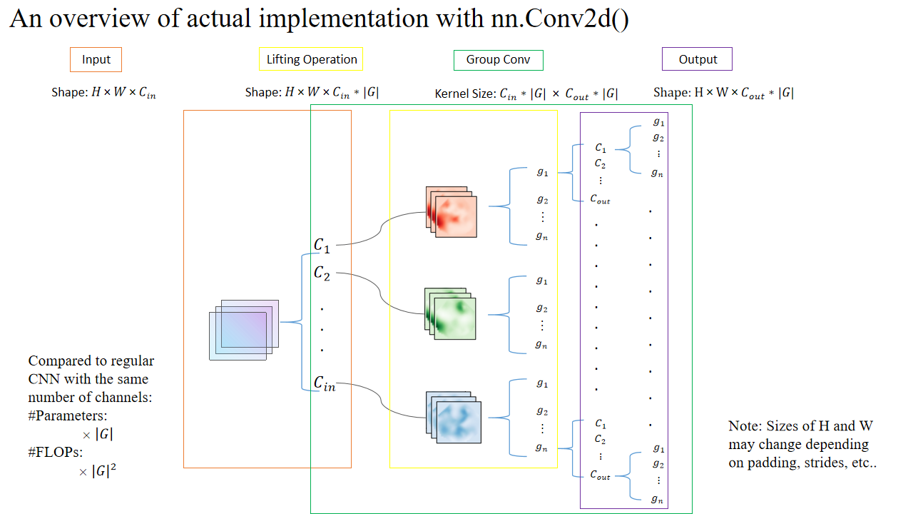
4.5. Overall Group CNN Pipeline

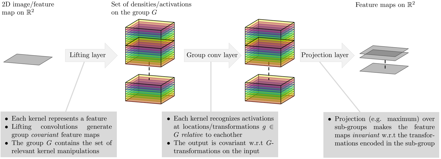
Overall, Group CNNs have the following structures:

1. Lifting Layer (Generate group equivariant feature maps):
   • 2D input $\Rightarrow$ 3D feature maps with the third dimension representing rotation.
2. Group Conv Layers (Convolve over the group space):
   • 3D feature maps $\Rightarrow$ 3D feature maps.
3. Projection Layer (Collapse the group dimension):
   • Invariance: 3D feature map $\Rightarrow$ 2D feature map by (e.g., max/avg) pooling over the $\theta$ dimension. Now, it is invariant in the $\theta$ dimension.
   • Equivariance: The resulting 2D feature map is rotation equivariant with respect to the input.

5. High-level Ideas on $SE(2)$ Steerable CNNs

5.1 From Group CNNs to Steerable CNNs

Group CNNs typically work with discrete groups of transformations, such as the $p_4$ group we have considered. However, many groups, including the rotation group, are continuous. You may perform very fine-grained discretization to capture the continuous nature of such groups, but the computational hurdle is intractable, and even so, discretizations still lose some of the continuity inherent in the group structure.

In a single sentence, steerable CNNs interpolate discrete (in terms of the rotation dimension) feature maps from group CNNs using Fourier/trigonometric interpolations.

• After the lifting layer, we have an extra dimension $\theta$ for the rotation angles. If we look at a specific pixel location, we can view all the feature values at this location as a periodic function $f: \theta \in [0, 2\pi) \mapsto \mathbb{R}$.

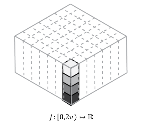
• How do we get continuous functions from discrete values? The answer is interpolation. As this function is periodic and defined on $[0, 2\pi)$, it is very natural to represent this function as a Fourier series. We can get the Fourier coefficients from discrete points, e.g., $0^\circ$, $90^\circ$, $180^\circ$, and $270^\circ$, by performing a discrete Fourier transform.

• Now, a periodic shift (translation) is a phase shift on these coefficients (Fourier shift theorem), and convolution is a point-wise multiplication with the coefficients.

• A little caveat: this is an approximation to equivariance if the degrees of rotation are not one of those discrete points.

For details, the readers are refered to [2].

References

[1] Group Equivariant Convolutional Networks by Taco S. Cohen and Max Welling

[2] Steerable CNNs by Taco S. Cohen and Max Welling

[3] Imperial’s Deep learning course: Equivariance and Invariance by Bernhard Kainz

[4] From Convolution to Neural Network by Gregory Gundersen

[5] UvA - An Introduction to Group Equivariant Deep Learning by Erik Bekkers

Other Useful Resources for Starters

Lecture Recordings

1. First Italian School on Geometric Deep Learning (Very nice mathematical prerequisites)
2. Group Equivariant Deep Learning (UvA - 2022)
3. Fourier Analysis by Steve Brunton

Survey Papers, Notes, and Books

1. Artificial Intelligence for Science in Quantum, Atomistic, and Continuum Systems (Section 2), Xuan Zhang (Texas A&M) et al.
2. Equivariant and Coordinate Independent Convolutional Networks: A gauge field theory of neural networks, Maurice Weiler el al.