Mean Flow (MF)

TL;DR: This write-up contains the minimum essential concepts and simple code to understand mean flow.

Readers are assumed to be familiar with flow matching: paper; tutorial.

The code follows the same style as the flow matching tutorial, using simple if–else statements to switch between flow matching (FM) and mean flow (MF) for easy transition and comparison.

The notebook version with the full code can be accessed here. If you have any questions or notice any errors, please contact me.

1. Problem Formulation

Given samples from two distributions $\pi_0$ and $\pi_1$, we aim to find a transport map $\mathcal{T}$ such that, when $X_0 \sim \pi_0$, then $X_1 = \mathcal{T}(Z_0) \sim \pi_1$.

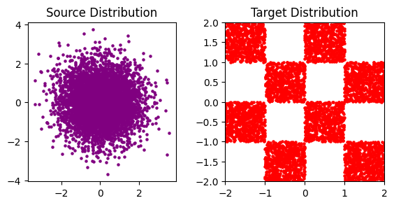
• $\pi_0$ is the source distribution, and $\pi_1$ is the target distribution.
• For image generation, $\pi_1$ can be the image data distribution and $\pi_0$ can be any prior distribution easy to sample from, e.g. Gaussian.

Code: We will use the standard Gaussian distribution as the source distribution and the “checkerboard distribution” as the target distribution. Let’s set up these two distributions.

def sample_pi_0(N=1000):
  return np.random.randn(N, 2).astype(np.float32)

def sample_pi_1(N=1000, grid_size=4, scale=2.0):
  return sample_checkerboard(N=N, grid_size=grid_size, scale=scale)

# Generate data
pi_0 = sample_pi_0(N=5_000)
grid_size, scale = 4, 2
pi_1 = sample_pi_1(N=5_000, grid_size=grid_size, scale=scale)

2. Background Information

Flow matching is introduced in this tutorial.

Notation:

• $\pi_0$: the source distribution
• $\pi_1$: the target distribution
• $X_0 \sim \pi_0$: random variables sampled from the source distribution
• $X_1 \sim \pi_1$: random variables sampled from the target distribution
• $\alpha_t=1-t$ and $\beta_t=t$: linear time schedule
• $X_t = t X_1+(1-t) X_0$: the flow interpolation
• $v_s\left(X_t, t\right) = X_1 - X_0$: the conditional velocity
• $\frac{d}{d t} X_t=v\left(X_t, t\right),t \in[0,1]$: the flow ODE
• $v\left(X_t, t\right)$: the marginal velocity

The flow matching objective is:

3. Mean Flow: One-step Generation

The learned velocity is marginal and non-constant, even with a linear schedule, so numerical solvers need many steps for accurate generation. Mean flow mitigates this issue by learning the average velocity over intervals instead of the instantaneous velocity $v\left(X_t, t\right)$.

The average velocity $u\left(X_t, r, t\right)$ over an interval $[r, t]$ with $t > r$ is defined as:

The goal is to train a neural network $u_\theta(X_t, t, r)$ to approximate $u$. With a good approximation, we can approximate the entire flow path using a single evaluation of $u_\theta(X_0, 0,1)$ (one-step generation).

We do not have $\int_{r}^{t} v(X_s, s) ds$ for training, so we manipulate this formulation a little:

Now, we can replace $u$ with $u_\theta$ and $v$ with $v_s=X_1-X_0$ for training.

4. JVP: Implicit Derivatives to Explicit Derivatives

Note that autograd can only directly compute explicit (partial) derivatives, while the time derivative is implicit ($u$ is a functional of a function of $t$). We apply multivariate chain rule:

where $\frac{d X_t}{d t} = v, \frac{d t}{d t} = 1$ and $\frac{d r}{d t} = 0$. This equation shows that the total derivative is given by the Jacobian-vector product (JVP) between $\left[\frac{\partial u}{\partial X_t}, \frac{\partial u}{\partial r}, \frac{\partial u}{\partial t}\right]$ (the Jacobian matrix of the function $u$ ) and the tangent vector $[v, 0,1]$. It can be efficiently computed by torch.func.jvp in PyTorch.

The training objective is:

where $r=\min \left(s_1, s_2\right), t=\max \left(s_1, s_2\right)$ with $s_1,s_2 \sim \text{Uniform (0,1)}$, $v_s = X_1- X_0$, and $X_t=t X_1+(1-t) X_0$.

Code: Let’s train the mean flow.

1. We setup the average velocity network $u_\theta$. We introduce an additional time variable $r$ for mean flow.

   class MLP(nn.Module): 
    def __init__(self, in_dim=2, context_dim=2, h=128, out_dim=2): 
        super(MLP, self).__init__()
        self.context_dim = context_dim
        self.network = nn.Sequential(nn.Linear(in_dim + context_dim, h), nn.GELU(),
                                     nn.Linear(h, h), nn.GELU(),
                                     nn.Linear(h, h), nn.GELU(),
                                     nn.Linear(h, h), nn.GELU(),
                                     nn.Linear(h, out_dim))
   
    def forward(self, x, t, r=None):
      if r == None:
        return self.network(torch.cat((x, t), dim=1))
      else: # mean flow takes an additional time r
        return self.network(torch.cat((x, t, r), dim=1))
   

2. We train the mean velocity network by randomly sampling $X_0, X_1$, $r$, and $t$, and minimizing the squared error above.

   def train_flow(flow_model, n_iterations=5_001, lr=3e-3, batch_size=4096, save_freq=1_000, flow="FM"):
    print(f"Training {flow}")
    optimizer = torch.optim.Adam(flow_model.parameters(), lr=lr)
    losses = []
    progress_bar = tqdm(range(n_iterations), desc="Training Flow Model", ncols=100)
    for iteration in progress_bar:
        x1 = torch.from_numpy(sample_pi_1(N=batch_size)).to(device)
        x0 = torch.from_numpy(sample_pi_0(N=batch_size)).to(device)
        if flow == "FM":
            t = torch.rand((x1.shape[0], 1), device=device) # randomly sample t
            x_t = t * x1 + (1.-t) * x0  
            v = x1 - x0  
            v_pred = flow_model(x_t, t)
            loss = torch.nn.functional.mse_loss(v_pred, v)
        elif flow == "MF":
            tr = torch.rand((x1.shape[0], 2), device=device)
            t = tr.max(dim=1, keepdim=True).values
            r = tr.min(dim=1, keepdim=True).values  
            x_t = t * x1 + (1.-t) * x0
            v = x1 - x0   # conditional velocity given the end points
            dtdt, drdt = torch.ones_like(t), torch.zeros_like(r)
            u_pred, dudt = torch.func.jvp(flow_model, (x_t, t, r), (v, dtdt, drdt))
            u_target = (v - (t - r) * dudt).detach()
            loss = torch.nn.functional.mse_loss(u_pred, u_target)
        else:
            raise NotImplementedError
    return flow_model, losses
   

5. Sampling with Learned Velocity

Once the velocity field $u_\theta\left(X_t, t, r\right)$ is learned, we can simulate samples from $\pi_1$ given samples from $\pi_0$ by:

One step generation can be achieved by:

def sample_flow(flow_model, N, T, flow="FM"):
    """
    Sample from pi_1 with the flow model in T time steps.
    """
    x = torch.from_numpy(sample_pi_0(N=N)).to(device)
    dt = 1./T
    for i in (range(T)):
        t = torch.ones((x.shape[0], 1), device=x.device) * (i * dt)
        if flow == "FM":
            pred = flow_model(x.squeeze(0), t) # predict v
        elif flow == "MF":
            r = t - dt
            pred = flow_model(x.squeeze(0), t, r) # predict u
        else:
            raise NotImplementedError
        x = x + pred * 1. / T # reverse integration as we learn the velocity from data to noise
    return x

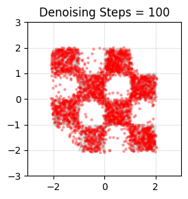
Generated Samples:

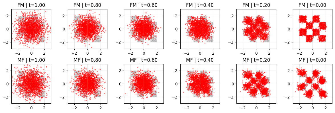
6. Mean Flow v.s. Flow Matching: One-step and Multi-step Generation

Let’s compare flow matching with mean flow under various sampling steps.

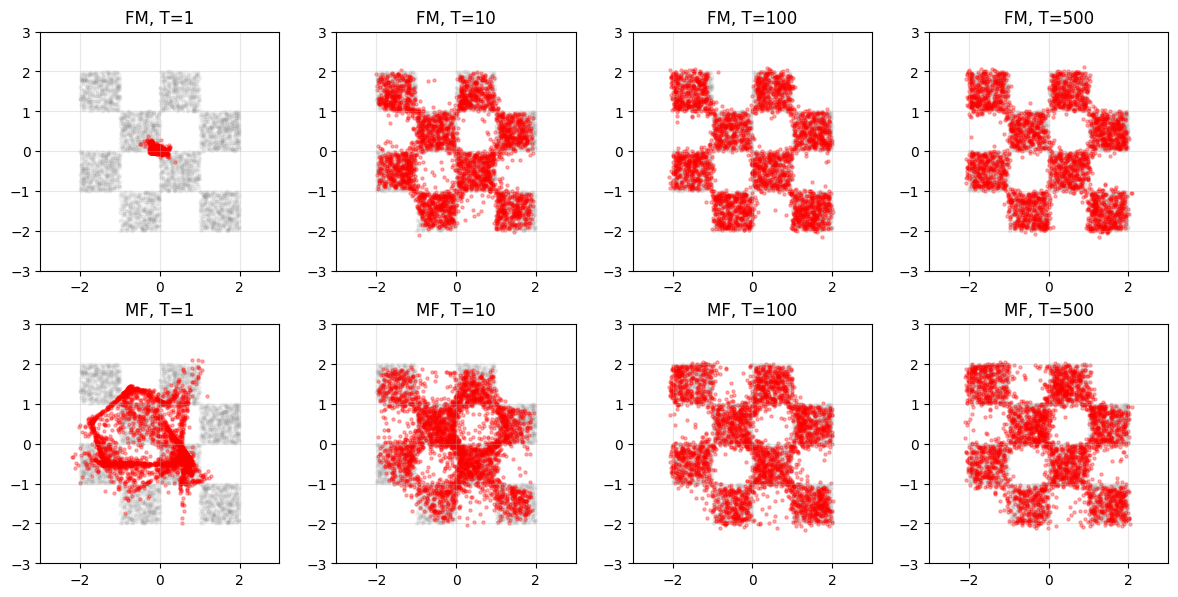
It can be seen that the 1-step generation of the mean flow is still poor. Flow models are often trained in the reverse direction for easier learning, so let’s try that.

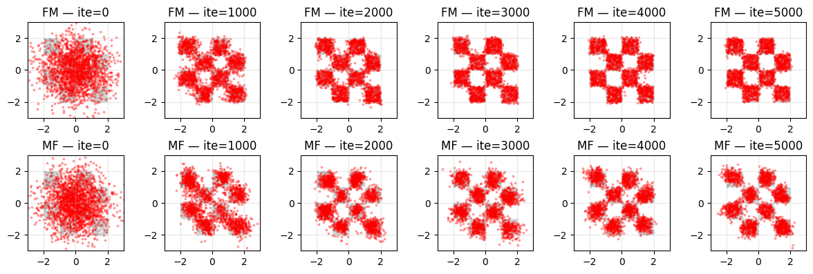
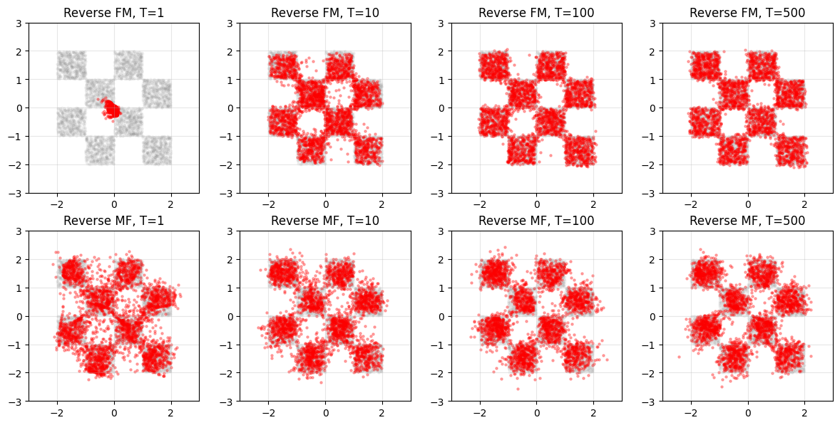
7. Reverse Training

As a common practice, instead of training a network to predict the “velocity” that moves noise → data, we instead train the network to predict the “velocity” that moves data → noise ($X_0$ is now data and $X_1$ is now noise). Then, at sampling time, we reverse the velocity field and integrate the ODE backward to recover samples from noise (use the negative velocity and integrate backward in time).

Code: Swap the two distributions.

def sample_pi_1(N=1000):
  return np.random.randn(N, 2).astype(np.float32)

def sample_pi_0(N=1000, grid_size=4, scale=2.0):
  return sample_checkerboard(N=N, grid_size=grid_size, scale=scale)
# Generate data
grid_size, scale = 4, 2
pi_0 = sample_pi_0(N=5_000, grid_size=grid_size, scale=scale)

Training is the same after swapping.

8. Reverse Integration

We perform reverse integration when $\pi_0$ is the target distribution. The time starts at 1, and we move along the negative velocity direction.

def sample_flow(flow_model, N, T, flow="FM", reverse=True):
    """
    Sample from pi_0 (checkboard) with the flow model in T time steps.
    """
    x = torch.from_numpy(sample_pi_1(N=N)).to(device)
    dt = 1./T
    for i in (range(T)):
        if reverse: # time starts from 1
          t = torch.ones((x.shape[0], 1), device=x.device) * (1 - i * dt)
        else: # time starts from 0 
          t = torch.ones((x.shape[0], 1), device=x.device) * (i * dt)
        if flow == "FM":
            pred = flow_model(x.squeeze(0), t) # predict v
        elif flow == "MF":
            r = t - dt
            pred = flow_model(x.squeeze(0), t, r) # predict u
        else:
            raise NotImplementedError
        x = x - pred * 1. / T if reverse else x + pred * 1. / T
    return x

9. Additional Visualization