Deep Generative Models

TL;DR: This blog provides an overview of (deep) generative models and a few foundational mathematical concepts.

1. Introduction

A statistical generative model is a probability distribution $p(x)$.

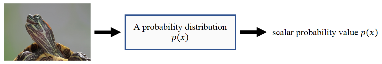
It is generative because sampling from $p(x)$ generates new data points.

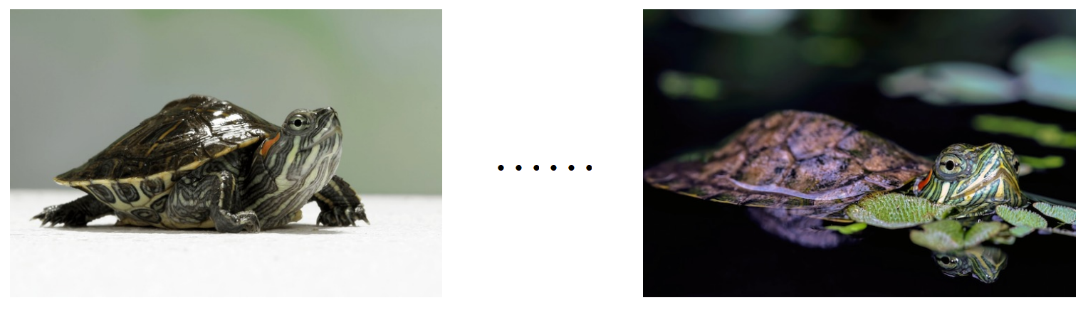
We are interested in learning the data distribution $p(x)$ with a model $p_\theta (x)$, parametrized by $\theta$, from an empirical dataset. The random variable $x$ represents a data sample drawn from the underlying data distribution $p(x)$. In some cases, we may not be able to explicitly model $p(x)$ directly but can instead just generate samples from it.

Example: Consider a data distribution of greyscale images, where \(x \in \mathcal{X}^D\), with \(\mathcal{X}=\{0,1, \ldots, 255\}\) representing the possible pixel intensity values, and $D$ the total number of pixels in each image. So, $p(x)$ represents the probability distribution over the space of all possible greyscale. In other words, $p(x)$ assigns a probability to each possible configuration of pixel values across the $D$ pixels.

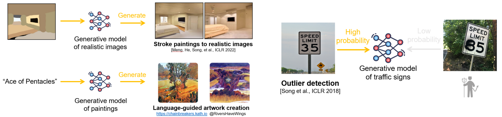
With probability distribution $p(x)$, we can do the following:

• Generation: Getting new samples from $p(x)$.
• Density Estimation: $p(x)$ should be high if $x$ is in distribution.
• Unsupervised Representation Learning: Learn what samples have in common; e.g. ears, hair colors, etc. for face images.

2. Useful Concepts and Mathematical Preliminaries

2.1. Control Signals

We often need some form of control signal (such as a latent variable $z$) for generation.

• High-dimensional data: Modeling the distribution $p(x)$ directly can be extremely difficult because the space of possible data points is vast and complex, requiring enormous amounts of data and may not generalize well.
• Latent structure: Data typically has underlying patterns and features. These latent factors are not directly observable in the data, but using a control signal allows the model to encode these underlying structures.

The data distribution $p(x)$ can then be factorized through the control signal $z$. It’s often useful to condition on rich information $z$.

\[p(x)=\int p(x \mid z) p(z) d z\]

The model splits the task of generating data into two parts:

1. Generating the latent variable $z$.
2. Generating a sample $x$ conditioned on $z$.

This allows the model to disentangle factors of variation in the data (e.g., shape, color, orientation) and represent them explicitly in the latent space.

2.2. Discriminative vs. Generative

Given a classification problem (discriminative), our goal is to learn the conditional probability of a sample belonging to a certain class, expressed as:

\[P(Y=c \mid X=x).\]

Given a generative problem, the input $X$ is not given. Requires a model of the joint distribution over both $X$ and $Y$. We are interested in learning the marginal probability \(P(X)\) or the joint probability ($Y$ as the control signal):

\[P(Y=c, X=x).\]

In summary:

• Discriminative: $X$ is always given, so there is no need to model $P(X)$; it cannot handle missing data or generate new data.
• We generate new $X$. Therefore, we need to model the complex distribution $P(X)$.

The conditional probability, marginal probability, and the joint probability are related by the Bayes’ Rule.

\[P(Y \mid X)=\frac{P(X \mid Y) P(Y)}{P(X)}=\frac{P(X, Y)}{P(X)}.\]

2.3. Concrete Example: Data Distribution

The MNIST consists of grayscale images with pixel values between $0$ and $255$. We can normalize them to $[0,1]$.

• Each MNIST image can be represented as a $784$-dimensional vector $(28 \times 28$ pixels $)$.
• After normalizing, each pixel’s value represents the probability that the pixel is on ($1$) or off ($0$). We model each pixel as an independent Bernoulli random variable.
• The joint distribution is the product of $784$ Bernoulli distributions:

\[p(x)=p \left( x _ 1, x _ 2, \ldots, x _ {784} \right) =\prod _ {i=1}^{784} p\left(x _ i\right)\]

Note: Obviously, pixels are not independent, but we make this assumption. Here, we assume Bernoulli distributions, however, you can use other distributions as well; Gaussian is another common choice. Later, we will discuss the log-likelihood and KL divergence of Bernoulli and Gaussian distributions, which will help clarify the rationale behind modeling images as Bernoulli or Gaussian variables.

2.4. Entropy, Cross-entropy, and KL Divergence

• Entropy $H(p)$ is a measure of the uncertainty in the distribution:

  \[H(p)=\mathbb{E} _ {X \sim p}[-\log p(X)].\]
  • Non-negativity: $H(p) \geq 0$, with equality if and only if $p$ is a degenerate distribution (all the probability mass is on one outcome).

• Cross-entropy $H(p, q)$ measures the expected number of bits needed to encode data from $p$ using the distribution $q$:

  \[H(p, q)=\mathbb{E} _ {X \sim p}[-\log q(X)].\]
  • Non-negativity: Cross-entropy is always non-negative.
  • Asymmetric: Cross-entropy is not symmetric, i.e., $H(p, q) \neq H(q, p)$.
  • Lower Bound: The cross-entropy $H(p, q)$ is greater than or equal to the entropy $H(p)$, i.e., $H(p, q) \geq H(p)$.
  • Equality: $H(p, q)=H(p)$ if and only if $p=q$, i.e., when the distributions are the same.

• KL Divergence $D _ {\mathrm{KL}}(p | q)$ : is a measure of how one probability distribution diverges from another:

  \[D _ {\mathrm{KL}}(p \| q)=\mathbb{E} _ {X \sim p}\left[\log \frac{p(X)}{q(X)}\right].\]
  • Non-negativity: $D _ {\mathrm{KL}}(p | q) \geq 0$, with equality if and only if $p=q$. This is a consequence of Jensen’s inequality.
  • Asymmetry: KL divergence is not symmetric, meaning $D _ {\mathrm{KL}}(p | q) \neq D _ {\mathrm{KL}}(q | p)$.
  • Relation to Cross-Entropy: The KL divergence can be expressed as the difference between the cross-entropy and the entropy:
  \[D _ {\mathrm{KL}}(p \| q)=H(p, q)-H(p).\]

2.5. Log-likelihoods and KL Divergence of Bernouli and Gaussian

Oftentimes, we assume a simple probability distribution $p(x)$ over the input. Common choices include (independent) Gaussian and Bernoulli. We are interested in learning a distribution parametrized by \(p _ \theta(x)\) through maximum likelihood learning or minimizing the KL divergence; here $\theta$ are the parameters of the distribution, which can be given by a neural network.

• Log Likelihood for Multivariate Bernoulli
  • For a multivariate Bernoulli distribution, the log likelihood of observing $x\in{0,1}^D$ or $x\in [0,1]^D$ is:
  \[p(x ; \theta) =\prod _ {i=1}^n \theta _ i^{x _ i}\left(1-\theta _ i\right)^{1-x _ i} .\]
  • The log-likelihood is:
  \[\log p(x ; \theta) =\sum _ {i=1}^n\left(x _ i \log \theta _ i+\left(1-x _ i\right) \log \left(1-\theta _ i\right)\right),\]

  where $\theta$ are the parameters of the bournoli distribution.

  This is essentially the form of the cross-entropy loss.

• Log Likelihood for Multivariate Gaussian
  • For a multivariate Gaussian distribution \(x \sim \mathcal{N}(\mu, \Sigma)\) with mean vector \(\mu \in \mathbb{R}^D\) and covariance matrix \(\Sigma \in \mathbb{R}^{D \times D}\) (that is \(\theta = [\mu,\Sigma]\)), the probability density function is given by:
  \[p(x ; \mu, \Sigma)=\frac{1}{(2 \pi)^{D / 2}|\Sigma|^{1 / 2}} \exp \left(-\frac{1}{2}(x-\mu)^{\top} \Sigma^{-1}(x-\mu)\right) .\]
  • Assuming $\Sigma$ is diagonal:
  \[p(x ; \mu, \Sigma)=\frac{1}{(2 \pi)^{D / 2} \prod _ {i=1}^D \sigma _ i} \exp \left(-\frac{1}{2} \sum _ {i=1}^D \frac{\left(x _ i-\mu _ i\right)^2}{\sigma _ i^2}\right) .\]
  • The log-likelihood is:
  \[\begin{aligned} \log p(x ; \mu, \Sigma) & =\log \left(\frac{1}{(2 \pi)^{D / 2} \prod _ {i=1}^D \sigma _ i}\right)-\frac{1}{2} \sum _ {i=1}^D \frac{\left(x _ i-\mu _ i\right)^2}{\sigma _ i^2} \\ & =-\frac{D}{2} \log (2 \pi)-\sum _ {i=1}^D \log \sigma _ i-\frac{1}{2} \sum _ {i=1}^D \frac{\left(x _ i-\mu _ i\right)^2}{\sigma _ i^2} \end{aligned}\]
  • The log-likelihood consists of $3$ terms:
    1. A constant term \(-\frac{D}{2} \log (2 \pi)\).
    2. A term that depends on the variances, \(-\frac{1}{2} \sum _ {i=1}^D \log \sigma _ i^2\).
    3. A term related to MSE that penalizes deviations from the mean, weighted by the inverse variances, \(-\frac{1}{2} \sum _ {i=1}^D \frac{\left(x _ i-\mu _ i\right)^2}{\sigma _ i^2}\).
• KL Divergence for Two Multivariate Gaussians
  • If \(p \sim \mathcal{N}\left(\mu _ p, \Sigma _ p\right)\) and \(q \sim \mathcal{N}\left(\mu _ q, \Sigma _ q\right)\), then
  \[KL\left(p\left(x ; \mu _ p, \Sigma _ p\right) \| q\left(x ; \mu _ q, \Sigma _ q\right)\right)=\frac{1}{2}\left(\log \frac{\left|\Sigma _ q\right|}{\left|\Sigma _ p\right|}-D+\operatorname{tr}\left(\Sigma _ q^{-1} \Sigma _ p\right)+\left(\mu _ q-\mu _ p\right)^{\top} \Sigma _ q^{-1}\left(\mu _ q-\mu _ p\right)\right) .\]
  • Assuming Diagonal Covariance Matrices:
  \[D _ {K L}\left(p\left(x ; \mu _ p, \Sigma _ p\right) \| q\left(x ; \mu _ q, \Sigma _ q\right)\right)=\frac{1}{2} \sum _ {i=1}^D\left(\log \frac{\sigma _ {q, i}^2}{\sigma _ {p, i}^2}-1+\frac{\sigma _ {p, i}^2}{\sigma _ {q, i}^2}+\frac{\left(\mu _ {p, i}-\mu _ {q, i}\right)^2}{\sigma _ {q, i}^2}\right).\]
  • The KL divergence consists of 3 terms:
    1. \(\frac{1}{2} \sum _ {i=1}^D \log \frac{\sigma _ {q, i}^2}{\sigma _ {p, i}^2}\): Accounts for the difference in variances.
    2. \(\frac{1}{2} \sum _ {i=1}^D \frac{\sigma _ {p, i}^2}{\sigma _ {q, i}^2}\): Measures the scaling difference in variances between the two distributions.
    3. \(\frac{1}{2} \sum _ {i=1}^D \frac{\left(\mu _ {p, i}-\mu _ {q, i}\right)^2}{\sigma _ {q, i}^2}\) : Penalizes differences in the means between $p$ and $q$ in terms of MSE, normalized by the variance of $q$.

  Note: If the variances in the Gaussian distributions are fixed (i.e., they are constants and not learnable parameters), then maximizing the log likelihood or minimizing the KL divergence between the true distribution and the predicted distribution reduces to optimizing the mean squared error (MSE) between the means of the distributions.

2.6. The Reparametrization Trick

When we want to optimize a function involving stochastic variables, we face an issue because gradients cannot directly flow through sampling operations.

• Specifically, consider an objective function $\mathcal{L}(\theta)$ that depends on a random variable $z$ sampled from a distribution parameterized by $\theta$:

\[\mathcal{L}(\theta)=\mathbb{E} _ {z \sim q _ \theta(z)}[f(z)].\]

• Our goal is to optimize $\theta$ (which can be given by a neural network, we can just back-propogate). For gradient-based optimization, we want to compute

\[\nabla _ \theta \mathcal{L}(\theta) = \nabla _ \theta \mathbb{E} _ {z \sim q _ \theta(z)}[f(z)].\]

• However, the sampling operation $z \sim$ $q _ \theta(z)$ introduces randomness that interrupts the gradient flow; another way to see this is that $z$ is not a deterministic function of $\theta$.

  • The issue arises because the sampled value $z$ is treated as a “constant” once sampled, and the gradient of a constant with respect to the distribution’s parameters $\theta$ is zero.

  • When you sample $z$ from a probability distribution $q _ \theta(z)$, like $z \sim \mathcal{N}\left(\mu, \sigma^2\right)$, the random variable $z$ is drawn based on the parameters $\theta=(\mu, \sigma)$ (mean and standard deviation). The sampling process itself is a discrete event, meaning once the sample $z$ is obtained, it becomes a fixed value.

    • Suppose $\mu=2, \sigma=1$, and you sample $z=2.5$.
    • Once $z=2.5$ is drawn, it’s just a fixed number. There’s no obvious relationship left between this fixed value $2.5$ and the parameters $\mu$ and $\sigma$ anymore.
    • The gradient of a constant with respect to any parameter is always zero:
    \[\nabla _ \mu z=0 \quad \text { and } \quad \nabla _ \sigma z=0.\]

• The reparameterization trick allows us to express the random variable $z$ as a deterministic function of the parameters $\theta$ and a separate random variable $\epsilon$.

  • Now, the randomness is removed, and $f$ can be written as a function of $\theta$, allowing gradient to flow.
    • $z=\mu+\sigma \cdot \epsilon, \epsilon \sim \mathcal{N}(0,1)$
    • The gradient is no longer zero:
    \[\nabla _ \mu z=\nabla _ \mu(\mu+\sigma \cdot \epsilon)=1 \quad \text { and } \quad \nabla _ \sigma z=\nabla _ \sigma(\mu+\sigma \cdot \epsilon)=\epsilon .\]
    • This enables the gradient to flow, allowing optimization of $f$ with respect to $\mu$ and $\sigma$.

Other Useful Resources for Starters

Books

Lecture Recordings

1. Stanford CS236 Deep Generative Models (2023)
2. A Course on Generative AI - Diffusion Models