Physics Informed Neural Networks (PINN) in 5 Minutes

TL;DR: This blog introduces the high level ideas of physics informed neural networks [1] in 5 minutes. A simple implementation to solve a Poission’s equation with both PINN and finite difference is also provided.

The toy implementation can be found here.

1. PINN Formulation

Consider the following general form of a PDE for $u(\boldsymbol{x})$ :

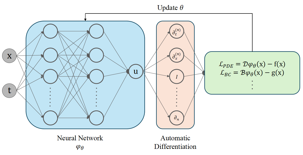
\[\begin{cases}\mathcal{D} u(\boldsymbol{x})=f(\boldsymbol{x}), & \text { in } \Omega, \\ \mathcal{B} u(\boldsymbol{x})=g(\boldsymbol{x}), & \text { on } \partial \Omega,\end{cases}\]

we wish to approximate $u(\boldsymbol{x})$ with a neural network, denoted by $\phi(\boldsymbol{x} ; \boldsymbol{\theta})$. We can train the neural network with physicsinformed loss. That is, we aim to solve the following optimization problem:

\[\boldsymbol{\theta}^*=\underset{\boldsymbol{\theta}}{\arg \min } \mathcal{L}(\boldsymbol{\theta}):=\underset{\boldsymbol{\theta}}{\arg \min } \underbrace{\|\mathcal{D} \phi(\boldsymbol{x} ; \boldsymbol{\theta})-f(\boldsymbol{x})\| _ 2^2} _ {\begin{array}{c} \text { Difference between the L.H.S. and } \\ \text { R.H.S. of the differential equation} \end{array}}+\lambda\|\mathcal{B} \phi(\boldsymbol{x} ; \boldsymbol{\theta})-g(\boldsymbol{x})\| _ 2^2.\]

The neural network takes spatio-temporal positions as inputs and produce the function value at these positions as outputs.
$\mathcal{D} \phi(\boldsymbol{x} ; \boldsymbol{\theta})$ can be approximated using the Monte Carlo method at collocation points.

Intuition: We penalize the neural network by the extend to which it violates the PDE/boundary/initial conditions. If the residual is exactly $0$, although nearly impossible, it means that $\phi(\boldsymbol{x} ; \boldsymbol{\theta})$ strictly satisfies the governing equations.

2. Sample Implementation

1. Use a feedforward neural network (fully connected network) to approximate the solution $u(x, y)$.

class FNN(torch.nn.Module): 
    def __init__(self, m):
        super(FNN, self).__init__()
        self.layer1 = nn.Linear(2, m)
        self.layer2 = nn.Linear(m, m)
        self.layer3 = nn.Linear(m, 1)
        self.activation = lambda x: tanh(x)

    def forward(self, tensor_x_batch):
        y = self.layer1(tensor_x_batch)
        y = self.layer2(self.activation(y))
        y = self.layer3(self.activation(y))
        y = y.squeeze(0)
        return y

2. Sample points in the domain and on the boundary, respectively.

def generate_points_in_the_domain(N_1):
    return torch.rand(N_1, 2)

def generate_points_on_the_boundary(N_2):
    num = -(-N_2//4)  # get ceil of N_2/4,
    zero_to_one = torch.rand(num, 1)
    # x1-x4 for 4 sides of the square, each num points
    x1 = torch.cat((zero_to_one, torch.zeros_like(zero_to_one)), dim=1)
    x2 = torch.cat((zero_to_one, torch.ones_like(zero_to_one)), dim=1)
    x3 = torch.cat((torch.ones_like(zero_to_one), zero_to_one ), dim=1)
    x4 = torch.cat((torch.zeros_like(zero_to_one), zero_to_one ), dim=1)
    x = torch.cat((x1, x2, x3, x4), dim=0)
    return x
	
x_1 = generate_points_in_the_domain(N_1)
x_2 = generate_points_on_the_boundary(N_2)

3. Calculate the Laplacian $\Delta u(x, y)$ (second derivatives with respect to $x$ and $y$ ) using automatic differentiation.

# calculate nabla u
def gradients(output, input):
    return autograd.grad(outputs=output, inputs=input,
                                grad_outputs=torch.ones_like(output),
                                create_graph=True, retain_graph=True, only_inputs=True)[0]
# get the partial derivatives ux and uy
nabla = gradients(network_solution_1, x_1)
# uxx + uyy
delta = gradients(nabla[:, 0],x_1)[:, 0] + gradients(nabla[:, 1], x_1)[:, 1]

4. Define the loss functions.

loss_1 = torch.mean(torch.square(delta - 5))
loss_2 = torch.mean(torch.square(network_solution_2 - 1))

5. Training the model to minimize the total loss, which is a combination of the residual and boundary losses (with a weighting term lambda).

loss = loss_1 + lambda_term * loss_2

Full implementation can be found here.

References

[1] Physics-informed neural networks: A deep learning framework for solving forward and inverse problems involving nonlinear partial differential equations, M. Raissi et al.