Operator Learning
TL;DR: This blog introduces a basic DeepONet (it has a lot of variants) [1] and its implementation.
The full implementation can be found here.
It is assumed that you are familiar with the basics of operator learning. If not, please read this first.
1. Introduction
DeepONet (Deep Operator Network) is a neural network designed to approximate operators $\mathcal{G}$, which are mappings from functions to functions:
\[\mathcal{G}: a(x) \mapsto u(y).\]DeepONet consists of two subnetworks:
- Branch Network: Encodes the input function $u(x)$ and produce \(\mathbf{b} \in \mathbb{R}^p\) as output.
- $b_1, b_2, \ldots, b_p$ serve as the function coefficients of the final output function.
- (Unstacked) Trunk Network: Represents a set of functions \(\{t_1, t_2, \ldots, t_p\}\).
- These functions serve as the function basis of the final output function.
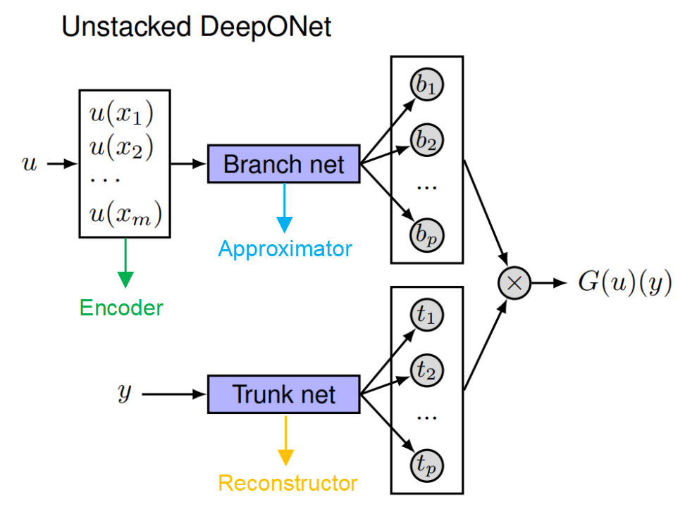
The final output is the assemble of the function coefficients and basis functions:
\[G _ \theta(u)(y) = \sum_{i=1}^p b_i t_i(y) = \underset{Branch}{\underbrace{\phi _ b\left(u(x _ 1),u(x _ 2),...,u(x _ m)\right)}} \odot \underset{Trunk}{\underbrace{\phi _ t(\textbf{y})}}.\]Note: If the basis functions are represented by MLPs, the output basis functions are naturally continuous (as implicit neural representations), so the output does not depend on the discretization of the data. However, the input functions must be observed at fixed sensor locations. FYI, some works have tried to address this limitation by learning the input function representation in a discretization independent manner, e.g. [2].
DeepONet is based on the universal approximation theory for operators:
Universal Approximation Theorem for Operators (Chen \& Chen, IEEE Trans. Neural Netw., 1995)
Suppose that \(\sigma\) is a continuous non-polynomial function, \(X\) is a Banach Space, \(K _ 1 \subset X, K _ 2 \subset \mathbb{R}^d\) are two compact sets in \(X\) and \(\mathbb{R}^d\), respectively, \(V\) is a compact set in \(C\left(K _ 1\right), G\) is a nonlinear continuous operator, which maps \(V\) into \(C\left(K _ 2\right)\). Then for any \(\epsilon>0\), there are positive integers \(n, p\), \(m\), constants \(c _ i^k, \xi _ {i j}^k, \theta _ i^k, \zeta _ k \in \mathbb{R}, w _ k \in \mathbb{R}^d, x _ j \in K _ 1, i=1, \ldots, n\), \(k=1, \ldots, p, j=1, \ldots, m\), such that
\[\vert G(u)(y)-\sum _ {k=1}^p \underbrace{\sum _ {i=1}^n c _ i^k \sigma\left(\sum _ {j=1}^m \xi _ {i j}^k u\left(x _ j\right)+\theta _ i^k\right)} _ {\text {branch }} \underbrace{\sigma\left(w _ k \cdot y+\zeta _ k\right)} _ {\text {trunk }}\vert<\epsilon\]holds for all \(u \in V\) and \(y \in K _ 2\).
2. Implementation
1. Define the DenseNet class for both branch and trunk networks (you can use other networks in practice, e.g. CNN-based networks for regular grid data)
class DenseNet(nn.Module):
    """
    A fully connected neural network (MLP) with ReLU activations between layers, except the last one.
    """
    def __init__(self, layers):
        super(DenseNet, self).__init__()

        self.n_layers = len(layers) - 1
        assert self.n_layers >= 1
        self.layers = nn.ModuleList()
        for j in range(self.n_layers):
            self.layers.append(nn.Linear(layers[j], layers[j+1]))
            if j != self.n_layers - 1:
                self.layers.append(nn.ReLU())

    def forward(self, x):
        for _, l in enumerate(self.layers):
            x = l(x)
        return x
2. The branch network takes the input function values at fixed sensor locations as input and the trunk network take spatiotemporal locations as input
class DeepONet(nn.Module):
    def __init__(self, branch_layer, trunk_layer):
        super(DeepONet, self).__init__()
        self.branch = DenseNet(branch_layer)
        self.trunk = DenseNet(trunk_layer)

    def forward(self, a, grid):
        b = self.branch(a)
        t = self.trunk(grid)
        return torch.einsum('bp,np->bn', b, t)

branch_layers = [250, 250, 250, 250, 250]
trunk_layers = [250, 250, 250, 250, 250]
model = DeepONet(branch_layer=[a_num_points] + branch_layers,
                   trunk_layer=[d] + trunk_layers).to(device)

# Note: a_num_points is the number of sensor locations for observing the input function a
# and u_dim is the spatiotemporal dimension of the output function u, e.g. 2 for 2D BVP (no time).
Full implementation can be found here.
References
[1] DeepONet: Learning nonlinear operators for identifying differential equations based on the universal approximation theorem of operators, Lu Lu et al.
[2] Operator learning with neural fields: Tackling PDEs on general geometries, Louis Serrano et al.