Geometric GNNs
TL;DR: This blog introduces geometric GNNs, which guarantee Euclidean (E(n)) symmetries in neural networks; for example, when you rotate a molecule, scalar quantities such as potential energy should remain invariant, and vector or tensor quantities should be equivariant to the rotation.
This tutorial aims to simplify abstract concepts for newcomers. Coding examples are provided to illustrate concepts including tensor decomposition, equivariance, and irreducibility.
- The toy implementation, along with some slides, can be found here.
- It is assumed that you are familiar with the basic concepts of equivariance. If not, please read Group CNN first.
- Reference [1] provides a great introduction to geometric GNNs. This blog will introduce geometric GNNs in less detail and focus on explaining tensor decomposition, the equivariance of tensors, and irreducibility.
1. Introduction
1.1. Geometric Representation of Atomistic Systems
There are different ways of representing molecules; for example:
- SMILES strings (1D)
- Planar graphs (2D)
- Geometric graphs (3D)
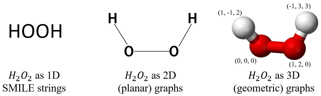
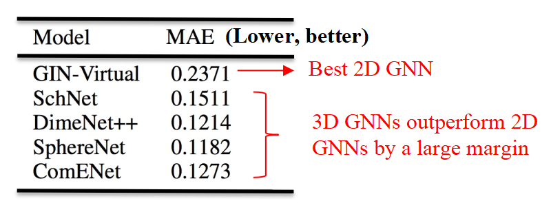
3D geometric configuration (coordinates) is crucial in determining properties and so, GNNs that learn with 3D representations outperforms their 2D counterparts by a large margin.
1.2. Graphs and Geometric Graphs
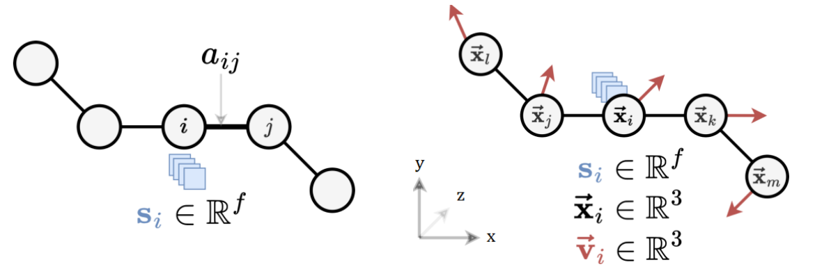
Graphs are purely topological objects and geometric graphs are a type of graphs where nodes are additionally endowed with geometric information.
| Graphs | Geometric Graphs |
| $G = (A,S)$ | $G = (A,S,X,V)$ |
| $A \in \mathbb{R}^{n \times n}:$ Adjacency matrix | $A \in \mathbb{R}^{n \times n}:$ Adjacency matrix |
| $S \in \mathbb{R}^{n \times f}$ : Scalar node features | $S \in \mathbb{R}^{n \times f}$ : Scalar node features |
| $X \in \mathbb{R}^{n \times 3}$ : $xyz$-coordinates | |
| $V \in \mathbb{R}^{n \times b \times 3}:$ Geometric features, e.g., velocity |
Here,
- Scalar loosely refers to features without geometric information.
- $n$ is the number of nodes, $f$ and $b$ are the sizes of the scalar and geometric node features, respectively.
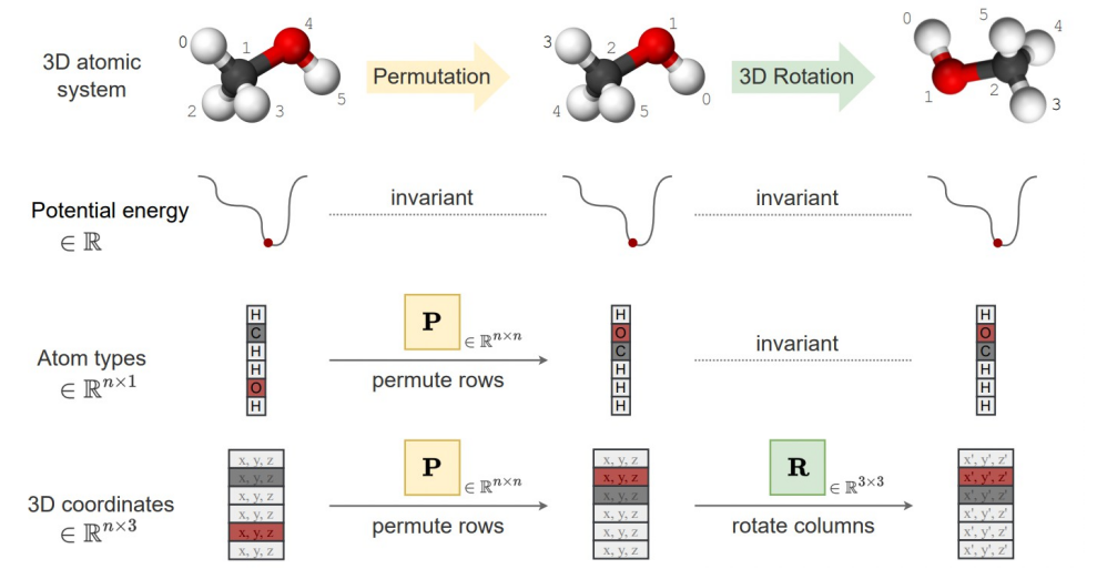
1.3. Symmetries
We have two types of features: scalar features and geometric features. We have the following symmetries:
- Scalar features remain unchanged (invariance).
- Geometric features transform with Euclidean transformations of the system (equivariance).
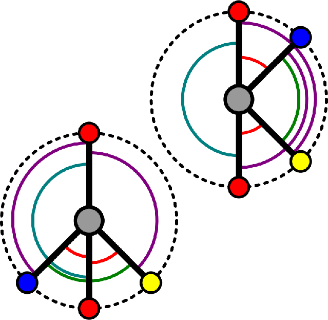
- Graphs,including geometric graphs, are permutationally equivariant node-wise and invariant graph-wise; it is still the same graph even if the nodes are given in a different order.
2. Geometric GNNs
2.1. GNNs and Geometric Message Passing
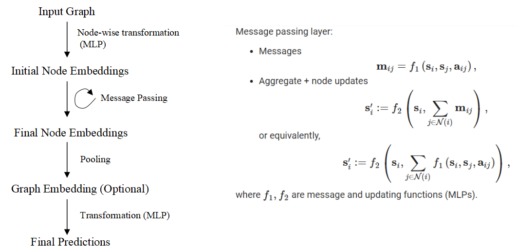
Graph Neural Networks (GNNs) are a class of deep learning models designed to operate on graph-structured data by learning node or graph representations through message-passing mechanisms to iteratively update node features to obtain useful hidden representations. In each layer, nodes aggregate information from their neighbors to update their features, allowing GNNs to effectively capture the relational and topological structure of graphs. GNNs are naturally permutation equivariant.
- Readers who are not familiar with GNNs are referred to Stanford CS224W: Machine Learning with Graphs.
For geometric message passing, we condition on geometries. Without loss of generality, let $a_{ij}$ contain geometric information for nodes $i, j$. We can have the following message passing schemes:
\[\mathbf{m}_{i j}=f_1\left(\mathbf{s}_i, \mathbf{s}_j, a_{ij}\right)\]To ensure symmetries
- Scalar features must be updated in an invariant manner.
- Geometric features must be updated in an equivariant manner.
Example: Let the relative position be the geometries and $f_1$ be an MLP, the messages $\mathbf{m}_{ij} = f_1\left(\mathbf{s}_i, \mathbf{s}_j, x_j - x_i\right)$ are clearly not equivariant.
To make it equivariant (invariant) to $E(3)$, there are in general two directions: Scalarization and Using Steerable Tensor Features. We term them as invariant GNNs and equivariant GNNs (Tensor Operations). Invariant GNNs constrain the geometric information that can be utilized, while the other constrains the model operations.
Scalarization GNNs (Invariant GNNs)
2.1. Summarization of Scalarization GNNs
Scalarization networks use invariant quantities as geometries that are conditioned. For example:
- Using relative distances (e.g. SchNet [2]):
- $\mathbf{m} _{i j}=f_1\left(\mathbf{s}_i, \mathbf{s}_j, d _{i j}\right)$, where $d _{i j}=\left|x_j-x_i\right|$
- $1$-hop, body order $2$, $O(nk)$ to compute invariant quantities with $n$ being the total number of nodes and $k$ being the average degree of a node.
- This is $E(3)$ invariant, but we limit the expressivity of the model as we cannot distinguish different local geometries.
- We cannot distinguish two local neighbourhoods apart using the unordered set of distances only.
- Using relative distances and bond angles (e.g. DimeNet [3]):
- $\mathbf{m}_ {i j}=f_1\left(s_ i, s_j, d_ {i j}, \sum_{k \in \mathcal{N}_j \backslash{i}} f_3\left(s_j, s_k, d _{ij}, d _{j k},\measuredangle i j k\right)\right)$
- $2$-hop, body order $3$, $O(nk^2)$ to compute invariant quantities
- This is $E(3)$ invariant, but again we limit the expressivity of the model due to similar reasons.
- Using relative distances, bond angles, and torsion angles (e.g. SphereNet [4]):
- $\boldsymbol{m} _ {i j}=f_1\left(s_i, s_j, d _ {i j}, \sum_{k \in \mathcal{N}_j \backslash{i}, l \in \mathcal{N}_k \backslash{i, j}} f_3\left(s_k, s_l, d _ {k l}, d _ {i j}, d _ {j k}, \measuredangle i j k, \measuredangle j k l, \measuredangle i j k l\right)\right)$
- $3$-hop, body order $4$, $O(nk^3)$ to compute invariant quantities
- This is $SE(3)$ invariant and complete, meaning that it can uniquely determine the 3D configuration of the geometric graph up to $SO(3)$ transformations (not $E(3)$ because reflections change the sign of torsions; you can make it $E(3)$ by ignoring the sign).
2.2. Pros and Cons
In summary, invariant GNNs update latent representations by scalarizing local geometry information. This is efficient, and we can achieve invariance with a simple MLP without specific constraints on the operations or activations we can take.
Pros:
- Simple usage of network architecture and non-linearities on many-body scalars.
- Great performance on some use cases (e.g., GemNet on OC20).
Cons:
- Scalability of scalar pre-computation. The accounting of higher-order tuples is expensive.
- Making invariant predictions may still require solving equivariant sub-tasks.
- May lack generalization capabilities (equivariant tasks, multi-domain).
3. Spherical Tensor GNNs (Equivariant GNNs)
3.1. Introduction
In invariant GNNs, invariants are ‘fixed’ prior to message passing. In equivariant GNNs, vector/tensor quantities remain available. Equivariant GNNs can also build up invariants ‘on the go’ during message passing. More layers of message passing can lead to more complex invariants being built up.
In invariant GNNs, we work with only scalars: $f\left(s_1, s_2, \ldots, s_n\right)$.
In equivariant GNNs, we work with scalars, vectors, and even high-order tensors: $f\left(s_1, s_2, \ldots s_n, \boldsymbol{v}_1, \ldots, \boldsymbol{v}_m\right)$.
Instantiation - “Scalar-vector” GNNs:
- Scalar message:
- Vector message:
where $\vec{x} _ {i j} = \vec{x} _ {j} - \vec{x} _ {i}$ denotes the relative position vector and $\odot$ denotes a scalar-vector multiplication.
Clearly, we can achieve equivariance while using geometric features $\mathbf{v}_i$-s and $\vec{x} _ {ij}$-s, but we have to constrain the model operations. The high-level idea is to keep track of the “types” of the objects and apply equivariant operations; we treat scalar and vector features separately and ensure that they maintain the same type through message passing.
As of now, we are constrained to have only scalar or vector features. What about higher-order tensors?
3.2. Cartesian Tensors and Tensor Products
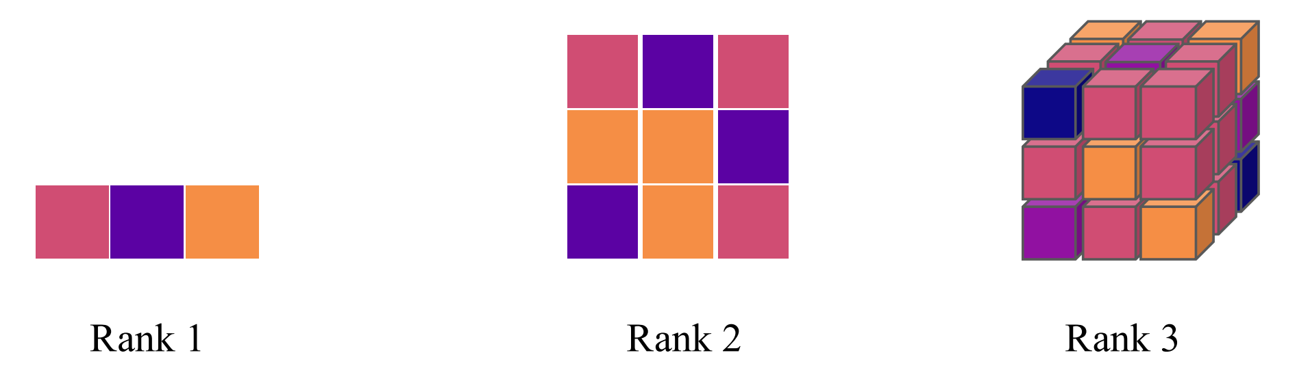
A tensor is a multi-dimensional array with directional information. A rank-$n$ Cartesian tensor $T$ can be viewed as a multidimensional array with $n$ indices, i.e., $T _ {\mathrm{i} _ 1 \mathrm{i} _ 2 \cdots \mathrm{i} _ n}$ with $i_k \in$ ${1,2,3}$ for $\forall k \in{1, \cdots, n}$. Furthermore, each index of $T _ {i_1 i_2 \cdots i_n}$ transforms independently as a vector under rotation.
- For a rotation represented by an orthogonal matrix $R$ , the components of $T$ transform as follows:
Equivalently, in index notation with Einstein summation convention, this can be written compactly as (refered to this StackOverflow Post for einsum operations):
\[T_{i_1^{\prime} i_2^{\prime} \cdots i_n^{\prime}}=R _ {i_1^{\prime} i_1} R _ {i_2^{\prime} i_2} \cdots R _ {i_n^{\prime} i_n} T _ {i_1 i_2 \cdots i_n}.\]A vector (rank-$1$ tensor) $v$ in 3D Euclidean space $\mathbb{R}^3$ can be expressed in the familiar Cartesian coordinate system in the standard basis:
\[\mathbf{e} _ x=\left(\begin{array}{l}1 \\\ 0 \\\ 0\end{array}\right) \mathbf{e} _ y=\left(\begin{array}{l}0 \\\ 1 \\\ 0\end{array}\right) \mathbf{e} _ z=\left(\begin{array}{l}0 \\\ 0 \\\ 1\end{array}\right).\]When you perform the tensor (or outer) product of two vectors in $\mathbb{R}^3$, you obtain a matrix (or a rank2 tensor). If you have two vectors
\[\mathbf{u}=\left(\begin{array}{c}u_x \\\ u_y \\\ u_z\end{array}\right) \text{ and }\mathbf{v}=\left(\begin{array}{c}v_x \\\ v_y \\\ v_z\end{array}\right),\]their tensor product $\mathbf{u} \otimes \mathbf{v}$ is given by:
\[\mathbf{u} \otimes \mathbf{v}=\left(\begin{array}{c} u_x \\ u_y \\ u_z \end{array}\right) \otimes\left(\begin{array}{c} v_x \\ v_y \\ v_z \end{array}\right)=\left(\begin{array}{lll} u_x v_x & u_x v_y & u_x v_z \\ u_y v_x & u_y v_y & u_y v_z \\ u_z v_x & u_z v_y & u_z v_z \end{array}\right)\]FYI: The definition of outer product of two functions: $(f \otimes g)(x, y)=f(x) g(y)$.
In terms of basis, if $\mathbf{u}$ and $\mathbf{v}$ are expressed in the standard basis ${\mathbf{e}_x, \mathbf{e}_y, \mathbf{e}_z}$, the resulting tensor product $\mathbf{u} \otimes \mathbf{v}$ can be viewed as a linear combination of the outer products of the basis vectors:
\[\begin{gathered} \mathbf{u} \otimes \mathbf{v}=u_x v_x\left(\mathbf{e}_x \otimes \mathbf{e}_x\right)+u_x v_y\left(\mathbf{e}_x \otimes \mathbf{e}_y\right)+u_x v_z\left(\mathbf{e}_x \otimes \mathbf{e}_z\right)+u_y v_x\left(\mathbf{e}_y \otimes \mathbf{e}_x\right)+u_y v_y\left(\mathbf{e}_y \otimes \mathbf{e}_y\right)+u_y v_z\left(\mathbf{e}_y \otimes \mathbf{e}_z\right)+u_z v_x\left(\mathbf{e}_z \otimes \mathbf{e}_x\right) \\ +u_z v_y\left(\mathbf{e}_z \otimes \mathbf{e}_y\right)+u_z v_z\left(\mathbf{e}_z \otimes \mathbf{e}_z\right) \end{gathered}\]The basis are given by:
\[\mathbf{e}_x \otimes \mathbf{e}_x=\left(\begin{array}{ccc} 1 & 0 & 0 \\ 0 & 0 & 0 \\ 0 & 0 & 0 \end{array}\right), \mathbf{e}_x \otimes \mathbf{e}_y=\left(\begin{array}{ccc} 0 & 1 & 0 \\ 0 & 0 & 0 \\ 0 & 0 & 0 \end{array}\right), \mathbf{e}_x \otimes \mathbf{e}_z=\left(\begin{array}{lll} 0 & 0 & 1 \\ 0 & 0 & 0 \\ 0 & 0 & 0 \end{array}\right), \mathbf{e}_y \otimes \mathbf{e}_x=\left(\begin{array}{ccc} 0 & 0 & 0 \\ 1 & 0 & 0 \\ 0 & 0 & 0 \end{array}\right), \ldots.\]3.3. Representations and Irreducibility
A representation $\rho: G \rightarrow G L(V)$ is a group homomorphism from G to the general linear group $G L(V)$. That is, $\rho(g)$ is a linear transformation parameterized by group elements $g \in G$ that transforms some vector $\mathbf{v} \in V$ (e.g. an image or a tensor) such that
\[\rho\left(g^{\prime}\right) \circ \rho(g)[\mathbf{v}]=\rho\left(g^{\prime} \cdot g\right)[\mathbf{v}].\]Example: The representation of $SO(3)$ acting on a geometric 3D vector is a $3 \times 3$ orthogonal matrices with determinant $1$.
A representation $\rho: G \rightarrow G L(V)$ is said to be irreducible if there are no proper non-zero subspaces $W$ of $V$ that are invariant under all group actions, i.e., $\rho(g) W \subseteq W$ for all $g \in G$. In other words, $V$ cannot be split into smaller subspaces that are individually invariant under the group action.
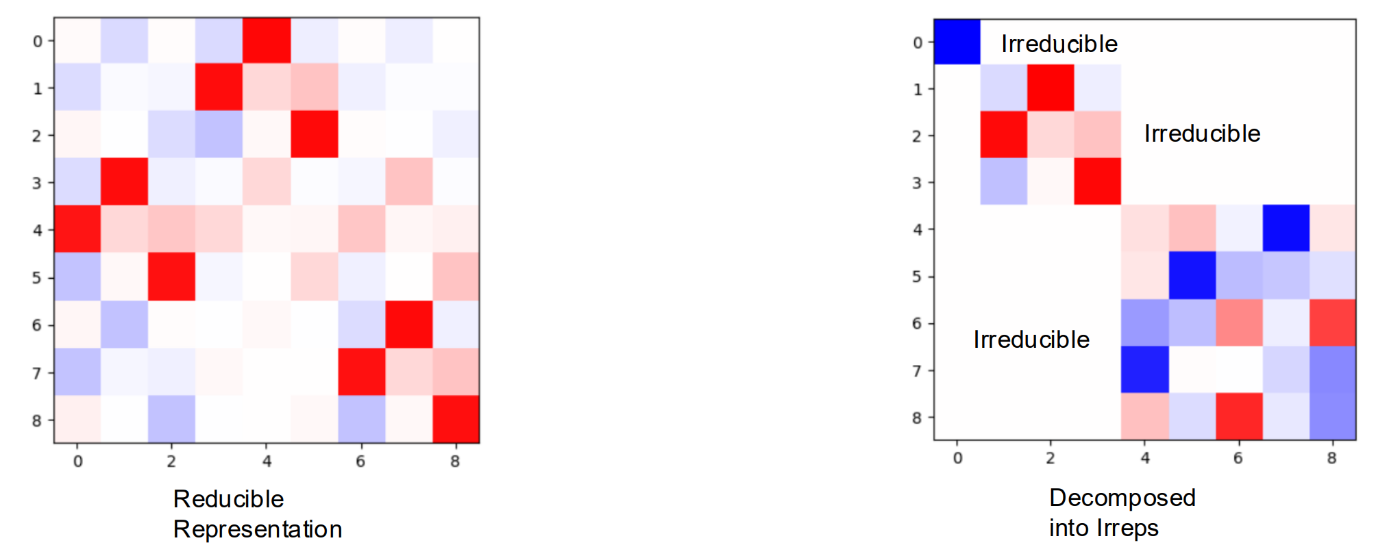
If a representation is reducible, it can be decomposed into a direct sum of irreducible representations (irreps). A block diagonal matrix can represent the direct sum of the matrices that lie along the diagonal. An irreducible representation cannot be decomposed further in this way.
Note: A block diagonal matrix does not necessarily indicate irreducibility; it might be further reduced or decomposed.
Irreducible representations are the “building blocks” of more complex representations. Representations are decomposed into indepedent simpler parts.
The representations of rotations for rank-$2$ Catersian tensors are generally reducible. Let $R$ be a rotation matrix for rank-$1$ Catersian tensors, we can write the representation on rank-$2$ Catersian tensors as $R_2 \in \mathbb{R}^{3\times 3\times 3\times3} = R \otimes R$. Here we losely abuse the notation $\otimes$ to denote $(A \otimes B) _ {i j, k l}=a_{i j} \cdot b _ {k l}$, it is more formally known as the Kronecker product. For details, refer to the implementation provided.
R_rank2 = torch.einsum('ij,kl', R, R)
plt.imshow(torch.kron(R, R), cmap='bwr', vmin=-1, vmax=1);
3.4. Decomposing Cartesian Tensors into Spherical Tensors
Now, as before, if we wish to maintain equivariance through message passing, we have to treat each rank separately. A general strategy is to treat each tensor as an entity and apply a single weight to it. However, the size of the tensor grows exponentially with the rank of the tensor, and it does not scale well. We can decompose the Cartesian tensor space into simpler parts (a direct sum of some subspaces).
- Each subspace acts independently under the actions of the rotation group (irreducible representations).
- Tensors in each subspace have the same “type”.
- Like scalar-vector networks, we apply equivariant operations to each type.

This process is a change of basis.
Change of Basis:
Let $\vec{v} \in V$ be a vector. Fix a basis ${e _ 1, \ldots, e _ n}$, whence you have $\vec{v}=\sum _ {i=1}^n e _ i v^i=\left(e _ 1, \ldots e _ n\right) \cdot\left(v^1, \ldots, v^n\right)^T$.
Then a change of basis is equivalent to the choice of an invertible $n \times n$ matrix $M$ via
$\vec{v}=\left(e _ 1, \ldots, e _ n\right) M M^{-1}\left(v^1, \ldots, v^n\right)^T=\left(\epsilon _ 1, \ldots, \epsilon _ n\right) \cdot\left(\nu^1, \ldots, \nu^n\right)^T$, where ${\epsilon _ 1, \ldots, \epsilon _ n}$ is the new basis and $\nu^1, \ldots, \nu^n$ are the new coefficients.
Note: Decomposition into irreps is not unique.
Specifically, we can decompose a Cartesian tensor of rank-$2$ as follows:
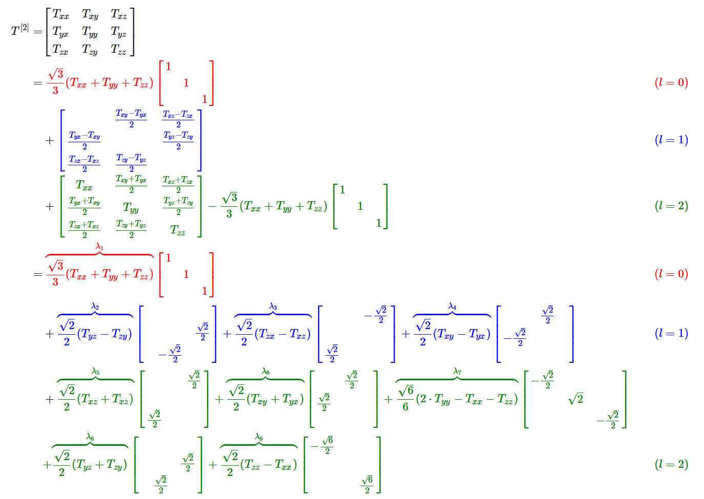
def decompose_tensor(T):
    if outer_product.shape != (3, 3):
        raise ValueError("Input must be a rank-2 tensor.")
    # l-0: Trace of the tensor
    l0 = np.trace(T) / np.sqrt(3)

    # l-1: Antisymmetric part
    antisymmetric_part = (T.T - T )/np.sqrt(2)
    l1 = np.array([
        antisymmetric_part[2, 1],  # T_yz - T_zy
        antisymmetric_part[0, 2],  # T_zx - T_xz
        antisymmetric_part[1, 0],  # T_xy - T_yx
    ])
    # l-2: Symmetric part
    symmetric_part = (T + T.T) /2
    matrix = symmetric_part.numpy()
    M_xx, M_yy, M_zz = matrix[0, 0], matrix[1, 1], matrix[2, 2]
    M_xy, M_xz, M_yz = matrix[0, 1], matrix[0, 2], matrix[1, 2]

    T_2m2 = M_xy* np.sqrt(2)                    # T_xy + T_yx
    T_2m1 = M_xz* np.sqrt(2)                    # T_xz + T_zx
    T_20 = (-M_zz - M_xx + 2* M_yy)/np.sqrt(6)  # 2T_yy - T_xx - T_zz
    T_21 = M_yz* np.sqrt(2)                     # T_yz + T_zy
    T_22 = (-M_xx + M_zz)/ np.sqrt(2)           # T_zz - T_xx
    l2 = np.array([T_2m1, T_2m2, T_20, T_21, T_22])
    return l0, l1, l2
For more details, refer to the implementation provided.
To summarize, we have seen that the $9$-dimensional rank-$2$ Cartesian tensor can be decomposed into $1d$, $3d$, and $5d$ parts:
$3 \otimes 3 = 1 \oplus 3 \oplus 5$.
These parts are called spherical tensors.
3.5. Spherical Tensor
A spherical tensor $T^\ell$ of order $\ell$ has $2 \ell+1$ components, denoted as $T_m^{\ell}$, where $m$ ranges from $-\ell$ to $\ell$. These components transform under rotations according to the rules of irreducible representations of the rotation group $S O(3)$.
If a rotation is represented by a matrix $R$, the components transform as:
\[{T}^{(\ell)} \rightarrow \mathcal{D}^{(\ell)}(\mathbf{R}) {T}^{(\ell)}\]where $\mathcal{D}^{(\ell)}(\mathbf{R})$ is the Wigner-$\mathcal{D}$ matrix of order $\ell$ for the rotation.
- Order-$0$ and rank-$0$ are the same (invariant under rotation).
- Order-$1$ and rank-$1$ are the same (transform under the normal $3 \times 3$ unitary rotation matrix).
3.6. Tensor Products of Spherical Tensors
Unfortunately, the tensor product of two spherical tensors ${S}^{\left(l_1\right)}$ and ${T}^{\left(l_2\right)}$ is generally not a spherical tensor anymore.
Example: As we have seen above, the tensor product of two $l_1$ spherical tensors ($9$ elements) is not an order-$4$ ($9$ elements) spherical tensor. We have to decompose it into spherical tensors of orders $0,1,2$.
However, we can decompose the tensor product ${S}^{\left(l_1\right)} \otimes {T}^{\left(l_2\right)}$ back into spherical tensors.
As a rule, the $\left(l_1 l_2\right)$-dimensional tensor product of two spherical tensors of ranks $l_1$ and $l_2$ decomposes into: \(l_1 \otimes l_2=\left|l_1-l_2\right| \oplus\left|l_1-l_2+1\right| \oplus \cdots \oplus\left(l_1+l_2-1\right) \oplus\left(l_1+l_2\right).\)
This means the $l_1 l_2$-dimensional product decomposes into exactly one spherical tensor for each rank between the absolute difference $\left\vert l_1-l_2\right\vert$ and the sum $l_1+l_2$.
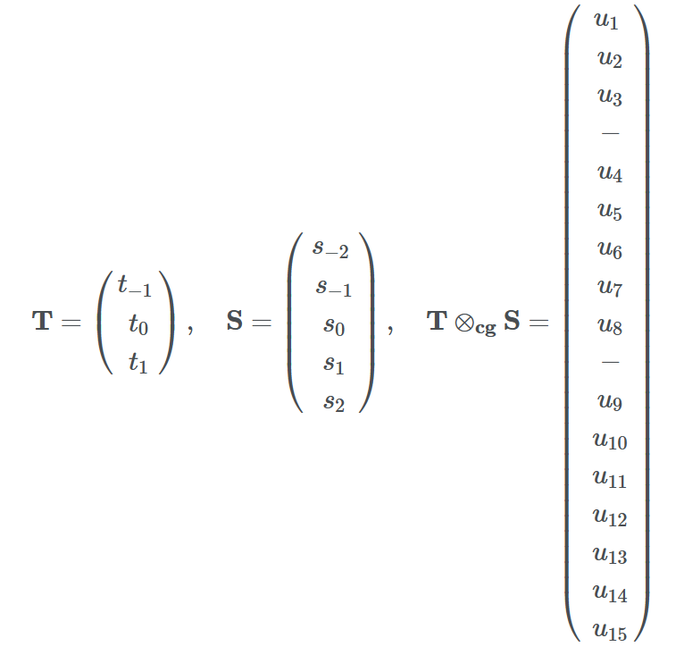
Example: $\vert1-2\vert= 1$ and $1+2 = 3$. The $15$ elements in the tensor product can be decomposed into a $l = 1$ ($3$ elements) tensor, a $l = 2$ ($5$ elements) tensor, and a $l = 3$ ($7$ elements). In some not so rigorous notation:$1 \otimes 2=1 \oplus 2 \oplus 3$.
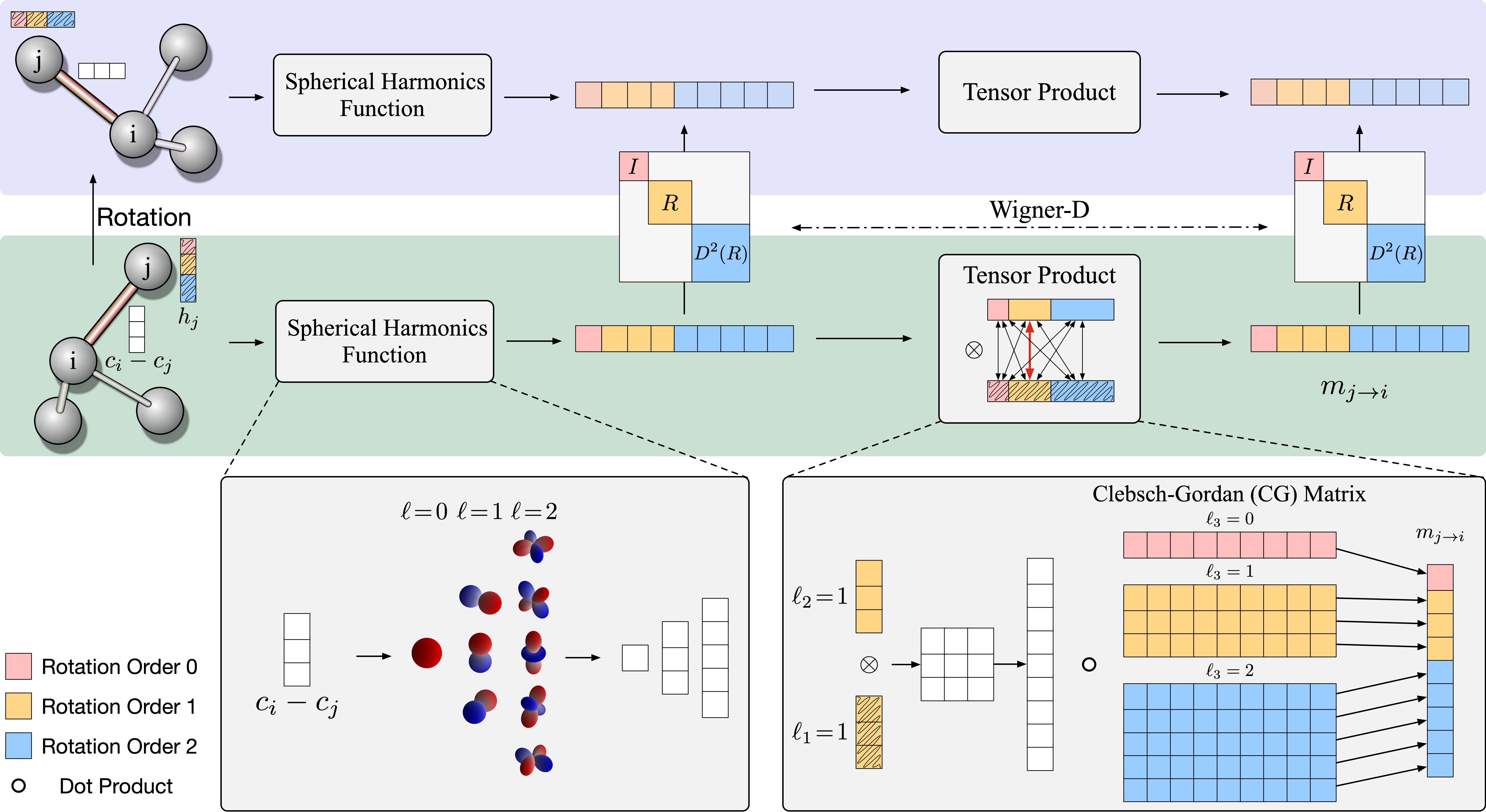
The coefficients of the decomposition (elements in the change of basis matrix) are given by the Clebsch-Gordan coefficients.
Example: Suppose we with to get the $l = 1$ tensor resulted from the tensor product of ${S}^{\left(l _ 1\right)} \otimes {T}^{\left(l _ 2\right)}$. Each of these three elements is a weighted sum of the $3\times 5$ resulting elements. So in total, we have $3 \times 5 \times 3 = 45$ coefficients. We denote this change of basis weights by $C _ {\left(m _ 1, m _ 2, m _ 3\right)}^{\left(l _ 1, l _ 2, l _ 3\right)}$, where $-\ell _ i \leq m _ i \leq \ell _ i$.
- $C _ {\left(m _ 1 =1, m _ 2 =2, m _ 3=1\right)}^{\left(l _ 1 =1, l _ 2 =2, l _ 3 =1\right)}$ means the coefficient of $t _ 1 \times s _ 2$ in order to get $u _ 1$ in the resulting tensor (We have $15$ coefficients for $u _ 1$).
- $u _ 1=\sum _ {i=-1}^1 \sum _ {j=-2}^2 C _ {\left(m _ 1=i, m _ 2=j, m _ 3=1\right)}^{\left(l _ 1=1, l _ 2=2, l _ 3=1\right)} t _ i s _ j$
- $u _ 2=\sum _ {i=-1}^1 \sum _ {j=-2}^2 C _ {\left(m _ 1=i, m _ 2=j, m _ 3=2\right)}^{\left(l _ 1=1, l _ 2=2, l _ 3=1\right)} t _ i s _ j$
- $u _ 3=\sum _ {i=-1}^1 \sum _ {j=-2}^2 C _ {\left(m _ 1=i, m _ 2=j, m _ 3=3\right)}^{\left(l _ 1=1, l _ 2=2, l _ 3=1\right)} t _ i s _ j.$ Similarly, $C _ {\left(m _ 1, m _ 2, m _ 3\right)}^{\left(l _ 1 =1, l _ 2 =2, l _ 3 =2\right)}$ will give the resulting $l=2$ tensor, etc..
3.7. Spherical Harmonics
Now we have a way to decompose tensor products into spherical tensors to keep track of and maintain the “types.” How do we get the tensors, other than $l_1$ (vectors), in the first place?
Real spherical harmonics $Y_l^m(\theta, \phi): S^2 \rightarrow \mathbb{R}$ are real-valued functions defined on the surface of a sphere.
\[Y_{\ell}^m(\theta, \varphi)=(-1)^m \sqrt{\frac{2 \ell+1}{4 \pi} \frac{(\ell-m)!}{(\ell+m)}} P_{\ell}^m(\cos \theta) e^{i m \varphi}\]Each real spherical harmonic is indexed by two integers: $l$ (degree) and $m$ (order), where $l \geq 0$ and $-l \leq m \leq l$. They are used as an orthonormal basis for representing functions on the sphere. Under fairly general condition (square-integrable on the sphere), any function can be written as a linear combination of spherical harmonics as follows:
\[f(\theta, \varphi)=\sum_{\ell=0}^{\infty} \sum_{m=-\ell}^{\ell} f_{\ell}^m Y_{\ell}^m(\theta, \varphi).\]
Generally, we can stack all the values from the degree-$l$ spherical harmonics together to get a order-$\ell$ spherical tensor.
\[V^{l=1} =\left(\begin{array}{l} Y _ {l=1}^{m=-1}(\theta, \phi) \\\ Y _ {l=1}^{m=0}(\theta, \phi) \\\ Y _ {l=1}^{m=1}(\theta, \phi) \end{array}\right)\]Example: Given a 3D point $v = (x,y,z)$, we can write it as a radial part $\Vert v \Vert$ and a directional part $\frac{v}{\Vert v \Vert}$. The directional part is now defined on $S^2$, write it as $(\theta, \phi)$. We can get a order-$1$ tensor with spherical harmonics as:
For simplicity, we can rewrite (real) spherical harmonics as a vector-valued function for order-$\ell$. That is $Y^{\ell}(\cdot): \mathbb{R}^3 \rightarrow \mathbb{R}^{2 \ell+1}$ maps an input 3D vector to a $(2 \ell+1)$-dimensional vector representing the coefficients of order- $\ell$ spherical harmonics bases.
Spherical harmonics function is equivariant to order-$\ell$ rotations, or so-called order-$\ell$ $S O(3)$ transformations: \(Y^{\ell}(R \boldsymbol{c})=D^{\ell}(R) Y^{\ell}(\boldsymbol{c}),\) where $\boldsymbol{c}$ is a 3D point.
Note: Spherical harmonics are a set of orthonormal functions defined on the surface of a sphere ($[0, \pi) \times [0, 2\pi)$) just like Fourier Basis. In fact, Fourier basis is called circular harmonics.
Summary of Terminology
Rank k Cartesian tensors: $T^{[k]}$
Order-$\ell$ Spherical tensors: $T^{(l)}$
Spherical jarmonics with degree $\ell$ and order $m$: $Y_l^m$
Order-$\ell$ Spherical harmonics function that gives the order-$\ell$ Spherical harmonics coefficients: $Y^{\ell}(\cdot)$
We have covered all the fundamental concepts in order to understand the overall pipeline of Spherical Tensor GNNs. The readers are refered to [1] and [5] for more detailed treatments.
References
[1] A Hitchhiker’s Guide to Geometric GNNs for 3D Atomic Systems, Duvel et al
[2] SchNet: A Continuous-filter Convolutional Neural Network for Modeling Quantum Interactions, Kristof T. Schütt et al.
[3] Directional Message Passing for Molecular Graphs, Johannes Gasteiger et al.
[4] Spherical Message Passing for 3D Graph Networks, Yi Liu et al.
[5] Artificial Intelligence for Science in Quantum, Atomistic, and Continuum Systems (Section 2), Xuan Zhang (Texas A&M) et al.
Other Useful Resources for Starters
Lecture Recordings
- First Italian School on Geometric Deep Learning (Very nice mathematical prerequisites)
- Group Equivariant Deep Learning (UvA - 2022)
Youtube Channels/Talks
- Graphs and Geometry Reading Group
- Euclidean Neural Networks for Learning from Physical Systems
- A Hitchhiker’s Guide to Geometric GNNs for 3D Atomic Systems
Architectures
- Geometric GNN Dojo provides unified implementations of several popular geometric GNN architectures