Unconstrained Methods for Symmetries

TL;DR: This blog introduces unconstrained methods for symmetries, taking the $E(3)$ group and point cloud data as an example.

This tutorial aims to simplify abstract concepts for newcomers. Coding examples are provided to illustrate PCA on point clouds, frame averaging, and equivariance.

The toy implementation, along with some slides, can be found here.
It is assumed that you are familiar with the Group CNN and Geometric GNNs. If not, please read them first.

1. Introduction

1.1. Motivation

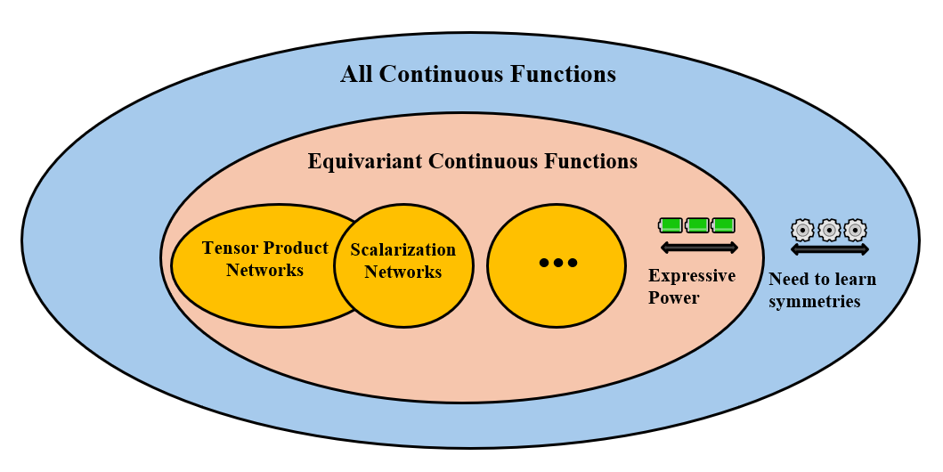
(Constrained) Geometric GNNs enforce symmetries directly into the architecture.

Restricting their set of possible operations or representations.
Hindering network capacity to fully express the intricacies of the data.
Computationally inefficient.
For large pretrained models, such as GPT, we cannot alter their network designs to ensure equivariance!

Does enforcing equivariance/symmetries as an inductive bias truly offset a potential reduction in optimization diversity within the constrained learning spaces?

It is desirable to have a pipeline in unconstrained learning spaces.

1.2. Group Averaging

Consider an arbitrary $\Phi: X \rightarrow Y$, where $X, Y$ are input and output (vector) spaces, respectively.

The GA operator $\langle\Phi\rangle _ G: X \rightarrow Y$ is defined as:

\[\langle\Phi\rangle _ G(x)=\mathbb{E} _ {g \sim \nu} \rho _ 2(g) \cdot \Phi\left(\rho _ 1(g)^{-1} \cdot x\right) = \int _ G \rho _ 2(g) \cdot \Phi\left(\rho _ 1(g)^{-1} \cdot x\right) d \nu(x),\]

or in summation form for discrete groups:

\[\langle\Phi\rangle _ G(x) = \frac{1}{\vert G \vert} \sum _ {g \in G} \rho _ 2(g) \cdot \Phi\left(\rho _ 1(g)^{-1} \cdot x\right).\]

$\rho _ 1(g), \rho _ 2(g)$: Group representations on $X$ and $Y$, respectively.
$\nu$: Harr measure over $G$ (“uniform” over $G$).

Claim: The GA operator is equivariant to $G$.
Proof:
$\begin{align*} \langle\Phi\rangle_G(h \cdot x) &= \mathbb{E}_{g \sim \nu} \rho_2(g) \cdot \Phi\left(\rho_1(g)^{-1} \cdot(\rho_1(h) \cdot x)\right) \\ &= \mathbb{E}_{g \sim \nu} \rho_2(g) \cdot \Phi\left(\rho_1\left(h^{-1} g\right)^{-1} \cdot x\right) \\ &= \rho_2(h) \mathbb{E}_{g \sim \nu} \rho_2\left(h^{-1} g\right) \cdot \Phi\left(\rho_1\left(h^{-1} g\right)^{-1} \cdot x\right) \\ &= \rho_2(h)\langle\Phi\rangle_G(x) \end{align*}$

Intuition: Similar to group convolutions, we have already calculated all the transformed versions of the input, $\rho_1(g)^{-1}x$ and $\rho_2(g)$ “corrects” the output for equivariance.

$\left\{\Phi\left(\rho_1(g)^{-1} \cdot x\right), \forall g\right\}$ will result in the same set of outputs, but in a different order, for transformed inputs.
- Why? Because the set of inputs $\left\{\rho_1(g)^{-1} \cdot x\right\}$ is the same but in a different order for a transformed $x$.
Thus, integrating/summing over these outputs will result in invariant outputs.
$\rho_2(g)$ “corrects” the output for equivariance by applying the transformation back.

Claim: GA is as expressive as its backbone $\Phi$ when $\Phi$ is equivariant to $G$.
Proof:
$\begin{aligned} \langle\Phi\rangle _ G(x) & =\mathbb{E} _ {g \sim \nu} g \cdot \Phi\left(g^{-1} \cdot x\right) \\ & =\mathbb{E} _ {g \sim \nu} g \cdot g^{-1} \cdot \Phi(x) \\ & =\Phi(x) \end{aligned}$

Opinion: When the backbone $\Phi$ is a general neural network, it is not equivariant. Therefore, this does not imply universal approximation of GA. In the case of FA (will introduce soon), it might even make the learning tasks more difficult.

Issue: When $\vert G \vert$ is large (e.g., combinatorial groups such as permutations), infinite (e.g., continuous groups such as rotations), or even non-compact, then the exact averaging is intractable.

1.3. Group Averaging and Group Convlution (Lifting)

Let $G = SO(2)$ be the proper rotation group on 2D images.

Recall the lifting operation:

\[[k \star f](g)=\int _ {\mathbb{R}^{\mathrm{d}}} k\left(g^{-1} y\right) f(y) d y=\left(L _ g \cdot k\right) \star f .\]

If we add the projection layer (average pooling layer) immediately, we have:

\[\langle\Phi\rangle _ G(f)=\mathbb{E} _ {g \sim \nu} L _ g \cdot\left[k \star\left(L _ g^{-1} \cdot f\right)\right]=\frac{1}{\vert G\vert } \sum _ {g \in G} L _ g \cdot\left[k \star\left(L _ g^{-1} \cdot f\right)\right]=\frac{1}{\vert G\vert } \sum _ {g \in G}\left(L _ g \cdot k\right) \star f .\]

Now, taking cross-correlation/convolution as the backbone function, the group averaging operator is defined as:

\[\langle\Phi\rangle _ G(f)=\mathbb{E} _ {g \sim \nu} L _ g \cdot\left[k \star\left(L _ g^{-1} \cdot f\right)\right]=\frac{1}{\vert G\vert} \sum _ {g \in G} L _ g \cdot\left[k \star\left(L _ g^{-1} \cdot f\right)\right]=\frac{1}{\vert G\vert} \sum _ {g \in G}\left(L _ g \cdot k\right) \star f .\]

They are essentially the same (with some caveats, see below). In group convolution, we modify the model architecture, making convolution kernels reflect the group ($L_g \cdot k$). In group averaging, we offset the symmetries to the input ($L_g^{-1} \cdot f$), and we additionally have the “correction term” as a result of this.

Claim: $k \star L_g f=L_g\left(L_g^{-1} k \star f\right)$ (We can move the rotation to images instead of on the kernel).
Proof:
$\begin{aligned} & {\left[\left(L _ g k\right) \star\left(L _ g f\right)\right](x) } \\ = & \int _ {\mathbb{R}^2} \operatorname{Lg} k(x-y) \operatorname{Lg} f(y) d y \\ = & \int _ {\mathbb{R}^2} k(g x-g y) f(g y) d y \\ = & \int _ {\mathbb{R}^2} k\left(g x-y^{\prime}\right) f\left(y^{\prime}\right) d y^{\prime} \\ = & \mathrm{Lg}(k \star f)(x). \end{aligned}$
Third equality: Change of variable $g y=y^{\prime}$ since the determinant of $g$ is $1$ (Caveat: $SO(2)$ is the special orthogonal group, but determinant of $1$ is not general).

def lift_correlation(image, kernel):
    """
    Apply lifting correlation/convolution on an image.

    Parameters:
    - image (numpy.ndarray): The input image as a 2D array, size (s,s)
    - conv_kernel (numpy.ndarray): The convolution kernel as a 2D array.

    Returns:
    - numpy.ndarray: Resulting feature maps after lifting correlation, size (|G|,s,s)
    """
    results = []
    for i in range(4):  # apply rotations to the kernel and convolve with the input
        rotated_kernel = np.rot90(conv_kernel, i)
        result = convolve2d(image, rotated_kernel, mode='same', boundary='symm')
        results.append(result)
    return np.array(results)
	
def group_averaging(image, kernel):
    """
    Apply group 'averaging' on an image, but do not average yet.

    Parameters:
    - image (numpy.ndarray): The input image as a 2D array, size (s,s)
    - conv_kernel (numpy.ndarray): The convolution kernel as a 2D array.

    Returns:
    - numpy.ndarray: Resulting feature maps before averaging, size (|G|,s,s)
    """
    results = []
    for i in range(4):  # apply inverse rotations to the images and convolve with the kernel
        rotated_image = np.rot90(image, 4-i)
        result = np.rot90(convolve2d(rotated_image, kernel, mode='same', boundary='symm'), i)
        results.append(result)
    return np.array(results)

Full code can be found here

2. Frame Averaging

2.1. Motivating Example: Geometric Pre-processing

Consider image segmentation, in which we want translation equivariance. Assuming we are using a model other than CNN, so that we do not have inherent translation equivariance, what can we do if we want translation equivariance? We can use group averaging, but it will be computationally intractable for the translation group (large in the discrete case or even infinite if we view it in a continuous manner). We should think of another way of achieving equivariance.

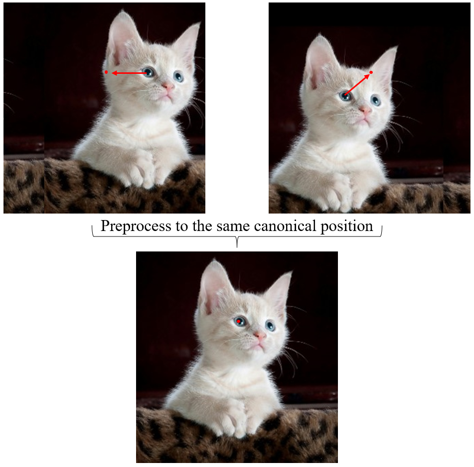
One way is geometric pre-processing:

Given an image, we can achieve equivariance by preprocessing the image.

For example, given cat images, if we have the location of the left eye of a cat, we can preprocess the image such that all cats will have their left eyes in the same location. Therefore, if an image is translated, it will be preprocessed to the same canonical position, eliminating the need for neural networks to have translation symmetries as these are accounted for in the data preprocessing (offset symmetries to the data).

2.2. Definition

A frame is defined as a set valued function $\mathscr{F}: X \rightarrow 2^G$ (Taking an input $x \in X$ and mapping it to a subset of $G$).

A frame is equivariant to $G$ if $\mathscr{F}(g \cdot x)=g \mathscr{F}(x), ∀g\in G$ (equality of sets).

The frame averaging operator [1] is defined as:

\[\langle\Phi\rangle _ {\mathcal{F}}(x)=\frac{1}{\vert \mathcal{F}(x) \vert} \sum _ {g \in \mathcal{F}(x)} \rho_2(g) \Phi\left(\rho_1(g)^{-1} x\right).\]

Similar to group averaging, we can prove that frame averaging operator is equivariant to $G$ if $\mathcal{F}$ is equivariant to $G$, and it is as expressive as its backbone if its backbone is equivariant.

Example: Consider $X=\mathbb{R}^n, Y=\mathbb{R^n}$, and $G=\mathbb{R}$ with addition as the group action.
We choose the group actions in this case to be $\rho_1(t) \boldsymbol{x}=\boldsymbol{x}+t \mathbf{1}$, and $\rho_2(a) y=y+t$, where $t\in G$, $\boldsymbol{x} \in X, y \in Y$ are point clouds of $n$ points, and $\mathbf{1} \in \mathbb{R}^n$ is the vector of all ones.
We can define the frame in this case using the averaging operator $\mathcal{F}(\boldsymbol{x})=\left\{\frac{1}{n} \mathbf{1}^T \boldsymbol{x}\right\} \subset G=\mathbb{R}$.
Note that in this case the frame contains only one element from the group (this special case when the frame size is $1$ is called canonicalization), in other cases finding such a small frame is hard or even impossible.
One can check that this frame is equivariant. The FA: $\langle\Phi\rangle _ {\mathcal{F}}(\boldsymbol{x})=\Phi\left(\boldsymbol{x}-\frac{1}{n}\left(\mathbf{1}^T x\right) \mathbf{1}\right)+\frac{1}{n} \mathbf{1}^T x$ in the equivariant case.
Intuition: Geometric pre-processing, we subtract the average (centroid) from the point cloud, then use any network to process them, and finally add the average back to obtain equivariance.

2.3.Practical Instantiation for $E(3)$ Group on 3D Point Clouds

Goal: We would like to incorporate Euclidean symmetry to existing permutation invariant/equivaraint point cloud networks (e.g. GNNs, Transformer without positional encodings, etc.).

Settings:

Input Space: $X=\mathbb{R}^{n \times 3}$ ($n$ nodes, each holding a $3$-dimensional vector as its position).
Group: $G=E(3)=O(3) \times T(3)$, namely the group of Euclidean motions in $\mathbb{R}^3$ defined by rotations and reflections $O(3)$, and translations $T(3)$.
Representation acting on $ \boldsymbol{x} \in X$: $\rho_1(g) \boldsymbol{x}=\boldsymbol{x} \boldsymbol{R}^T+\mathbf{1} \boldsymbol{t}^T$, where $\boldsymbol{R} \in O(3)$, and $\boldsymbol{t} \in \mathbb{R}^3$. (Apply rotation and translation to every node).
Output space $Y$ and representation acting on the output space $\rho_2$ are defined similarly.

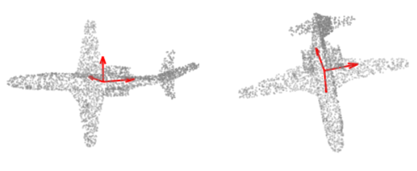
Frame $\mathcal{F}(\boldsymbol{x})$ is defined based on Principle Component Analysis (PCA), as follows:

Let $\boldsymbol{t}=\frac{1}{n} \boldsymbol{x}^T \boldsymbol{1} \in \mathbb{R}^3$ be the centroid of $\boldsymbol{x}$
$\boldsymbol{C}=\left(\boldsymbol{x}-\mathbf{1} \boldsymbol{t}^T\right)^T\left(\boldsymbol{x}-\mathbf{1} \boldsymbol{t}^T\right) \in \mathbb{R}^{3 \times 3}$ the covariance matrix computed after removing the centroid from $\boldsymbol{x}$. In the generic case the eigenvalues of $\boldsymbol{C}$ satisfy $\lambda _ 1<\lambda _ 2<\cdots<\lambda _ 3$.
Let $\boldsymbol{v} _ 1, \boldsymbol{v} _ 2, \ldots, \boldsymbol{v} _ 3$ be the unit length corresponding eigenvectors.
Then we define $\mathcal{F}(\boldsymbol{x})=\left\{\left(\left[\alpha _ 1 \boldsymbol{v} _ 1, \ldots, \alpha _ 3 \boldsymbol{v} _ 3\right], t\right) \mid \alpha _ i \in\{-1,1\}\right\} \subset E(3)$. The frame size is $8$.
$\left[\boldsymbol{v} _ 1, \ldots, \boldsymbol{v} _ 3\right]$ is a set of orthonormal vectors in $\mathbb{R}^{3}$, i.e., a basis of $\mathbb{R}^{3}$. Moreover, these vectors will “rotate” in the same way as the input.
$\mathcal{F}(\boldsymbol{X})$ based on the covariance and centroid are $E(3)$ equivariant.

Principle directions rotate as the point cloud rotates. Frames based on PCA are equivaraint.

Note: We can reduce the frame size from $8$ to $4$ if we know the rotations are proper rotations (determinant is strictly $1$). This can generalize to any dimension $d$ beyond $3$, with frame size $2^d$ for the $O(d)$ group and $2^{d-1}$ for the $SO(d)$ group.

def getting_principal_directions(point_cloud):
    cov_matrix = np.cov(point_cloud, rowvar=False)
    eigenvalues, eigenvectors = np.linalg.eigh(cov_matrix)
    sorted_indices = np.argsort(eigenvalues)[::-1]
    principal_directions = eigenvectors[:, sorted_indices].T
    return principal_directions
	
def getting_frames(principal_directions):
    # Given the principal directions in 3D, output all 8 possibilities (sign ambiguity)
    frames = []
    for signs in np.array(np.meshgrid([-1, 1], [-1, 1], [-1, 1])).T.reshape(-1, 3):
        frames.append(principal_directions *signs[:, np.newaxis])
    return np.array(frames)
	
def FA(point_cloud, principal_directions, f): # f can be any function, does not have to be equivariant
    frames = getting_frames(principal_directions)
    inverse_frames = np.linalg.inv(frames)
    rho1_point_cloud = np.einsum('ijk,nk->inj', frames, point_cloud) # using the axes represented by principal vectors -> applying inverse rotation
    f_rho1_point_cloud = f(rho1_point_cloud)
    rho2_f_rho1_point_cloud = np.einsum('ijk,ink->inj', inverse_frames, f_rho1_point_cloud)